Forum Discussion
I need help with my excel file. Nested If statements
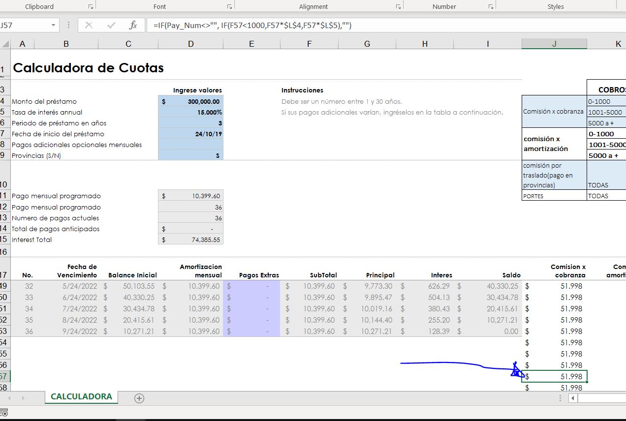
In the Column: Comision x cobranza
I want the column to update the numbers along with the No. column
for example --- I thought this might be a solution
=IF(Pay_Num<>"",if(F18<1000,F18*$L$4,F18*$L$5,"")
but I'm struggling with this. As you can see the column Comision x cobranza doesn't update with the values of the calculator and I need it to.
3 Replies
- SergeiBaklanDiamond Contributor
I didn't find where do you use this formula, but in any case it's incorrect. It could be
=IF(@Pay_Num<>"", IF(F18<1000,F18*$L$4,F18*$L$5) ,"")Pay_Num is the range, better to use cell reference in the formula.
Plus you have circular references in your file, better to find and remove.
 Michael_Epstein123Copper Contributor
thank you for the response. It helped me out one little step, but the excel file still isn't doing what I really want it to do yet.
look at this picture...
I want the cells in the J column to grow or shrink in number of rows in accordance with the A column
Does that make sense? Like if the Loan term is 24 payments (for 2 years).. I don't want J column to show 330 rows. I want it to show 24 rows in accordance with the A column!
Make sense?
SergeiBaklan Thank you for the help though. It's getting there. I'm just not sure how to describe this better and i'm unsure of how to make excel automate this;. view the screenshot
- Riny_van_EekelenPlatinum Contributor
The problem is caused by the fact that the cells with all the @-formulae are not recognised as blanks. Testing for a blank in A always seems to come up as a FALSE.
Leaving the logic of your sheet intact you can resolve it by first changing the payment counter. Keep A18 as is as it starts your calculations as soon as data is entered in the top of the schedule. But in A19 (and downwards) you could enter:
=IF(ROUND(I41,0)=0,"",A41+1)
It checks if the rounded previous balance ("Saldo") was zero. If so, it enters a blank. If not, it increases the payment number by 1.
In J18, L18 and M18 (and down) you could enter:
=IF(ISNUMBER(A18),IF(F18<1000,F18*$L$4,F18*$L$5),"")
=IF(ISNUMBER(F18),IF($D$9="S",F18*$L$10,0),"")
=IF(ISNUMBER(F18),F18+J18+K18+L18+$L$11,"")
The ISNUMBER part just checks that certain cells contain numbers, to avoid a #VALUE errors when you try to calculate with them.
I tested it and it seems to work as you want it to. And.... I don't get the circular reference notice anymore upon opening the schedule. Am attaching my version of your workbook for your information.