Oct 12 2021 10:55 AM
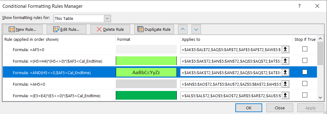
Hi everyone! I need a little help with conditional formatting, everything I've tried has not worked.
I am working on a schedule output excel sheet, were the scheduling information is entered on one tab and it outputs a nice looking schedule on a different tab. I used a template to get started and have been able to adjust everything to make it work except for the conditional formatting.
The template used an index/match formula to pull over values, and the conditional formatting makes it so that sometimes the values show and other times they are hidden (same background/font color). I love everything except I would like the "shown values" to be different colors based on the content of cell, I'm using "FIT" for this example. (see attached screenshots for schedule and conditional formatting.)
I have tried adding to the "and" function (this is the existing formula =AND(H5<>0,$AF5<Cal_Endtime)) in the formatting to include all of the following, but it hasn't worked:
The things I've added work on their own, but do not work when combined in any of these ways with the above format. Any advice would be very much appreciated!
Oct 12 2021 12:21 PM
@gabepatten
You need to wrap your ANDs in an IF like this:
=IF(AND(AH5="FIT",AND(H5<>0,$AF5<Cal_Endtime)),TRUE,FALSE)
Oct 12 2021 02:00 PM
Oct 12 2021 02:01 PM
@edawcj updated screenshot.. where did I go wrong?