Forum Discussion
Conditional Formatting, multiple conditions
Hi everyone! I need a little help with conditional formatting, everything I've tried has not worked.
I am working on a schedule output excel sheet, were the scheduling information is entered on one tab and it outputs a nice looking schedule on a different tab. I used a template to get started and have been able to adjust everything to make it work except for the conditional formatting.
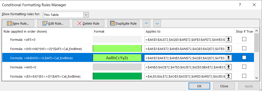
The template used an index/match formula to pull over values, and the conditional formatting makes it so that sometimes the values show and other times they are hidden (same background/font color). I love everything except I would like the "shown values" to be different colors based on the content of cell, I'm using "FIT" for this example. (see attached screenshots for schedule and conditional formatting.)
I have tried adding to the "and" function (this is the existing formula =AND(H5<>0,$AF5<Cal_Endtime)) in the formatting to include all of the following, but it hasn't worked:
- =AND(AH5="FIT",H5<>0,$AF5<Cal_Endtime)
- =AND(AH5="*FIT*",H5<>0,$AF5<Cal_Endtime)
- =AND(ISNUMBER(FIND("FIT",AH5)),H5<>0,$AF5<Cal_Endtime)
The things I've added work on their own, but do not work when combined in any of these ways with the above format. Any advice would be very much appreciated!
3 Replies
- edawcjBrass Contributor
gabepatten
You need to wrap your ANDs in an IF like this:=IF(AND(AH5="FIT",AND(H5<>0,$AF5<Cal_Endtime)),TRUE,FALSE) gabepattenCopper Contributor
- gabepattenCopper Contributor