Forum Discussion
smo4142
Jul 25, 2019Copper Contributor
Unable to edit source list in data validation in Excel
Hello, I have a created a drop down list in Excel 2016 and would like to edit the source list. However, when I go the source list under the data validation type and try to move across the list, it p...
- Feb 24, 2022
OK, then the formula needs to filter the matching dates and sum their amounts.
Since it seems you have one date per section you will probably do best using the versions that are one formula per answer in b29:b32
=LET(dateCell; A29; dateAnchor; Sheet2!$F$3; valueAnchor; Sheet2!$G$3; allValues; valueAnchor:endDown(valueAnchor); allDates; dateAnchor:endDown(dateAnchor); foundValues; FILTER(allValues;allDates=dateCell); output; SUM(foundValues); IFERROR(output;0) )
b1 and b18 do about the same but spills the result to dates below.
-/-
> If a person changes the Date column filter to just show Feb 22, why does it not change the running totals to reflect just that date?
The quite new function filter excludes data from calculation.
The command filter affects what is displayed on the screen - the hidden data is still there and included in calculations.
If you'ld like to show only the displayed subtotal you could use the function subtotal(9;range) instead of sum(range) but that is apart from the above solution.
Haytham Amairah
Jul 25, 2019Silver Contributor
Hi,
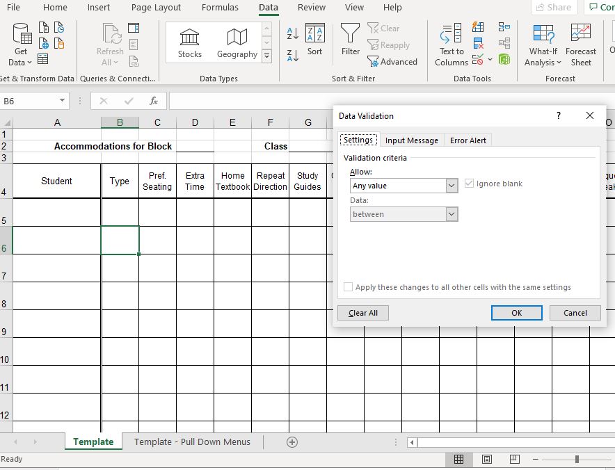
When you go to the Source box in the Data Validation and you want to edit it, you need to switch to the Edit mode.
The default is the Enter mode as the below screenshot:
Just press F2 to switch to the Edit mode so that you can move the cursor without inserting any cell references.
Hope that helps
- NikolinoDEJan 20, 2024Gold Contributor
You can achieve this by using a combination of Excel functions and conditional formatting.
Here is a step-by-step guide:
Assuming your jobs are listed in the range AO1:XX1 and the job entries are in the range D5:D370, you can follow these steps:
Step 1: Create a Helper Column
- Create a helper column (for example, column E) next to your job entries (D5:D370).
- In cell E5, enter the following formula:
=MATCH(D5,$AO$1:$XX$1,0)
Drag this formula down for the entire range (E5:E370). This formula will return the position of the job in the header row.
Step 2: Apply Conditional Formatting
- Select the range D5:D370.
- Go to the "Home" tab on the ribbon.
- Click on "Conditional Formatting" in the toolbar.
- Choose "New Rule" from the drop-down menu.
- Select "Use a formula to determine which cells to format."
- In the formula box, enter the following formula:
=E5<>"" (or =NOT(ISBLANK(E5)) if you want to cover empty cells)
This formula checks if the helper column has a value (i.e., a job is listed in that hour).
- Click on "Format" and set your desired background color under the "Fill" tab.
- Click "OK" to apply the formatting.
- Click "OK" again in the New Formatting Rule dialog.
Step 3: Apply Formatting to the Header Row
- Select the range AO1:XX1.
- Repeat steps 4-11, using the same formula:
=MATCH(AO1,$AO$1:$XX$1,0)<>"" (or =NOT(ISBLANK(MATCH(AO1,$AO$1:$XX$1,0))) for empty cells)
This formula checks if the job name is listed in the helper column.
Notes:
- The text and steps were edited with the help of AI.
- The helper column is used to match the job names between the header and the entries.
- The conditional formatting formula checks if the corresponding cell in the helper column has a value, and if so, applies the formatting.
- This setup dynamically adjusts to new job entries without the need for manual adjustments in conditional formatting rules.
Remember to adjust the cell references based on your actual data if needed.
My answers are voluntary and without guarantee!
Hope this will help you.
Was the answer useful? Mark as best response and Like it!
This will help all forum participants.
- FFAMATOJan 20, 2024Copper Contributor
Thank you all.
sorry, i gave you a wrong information before and only noticed now,
the second range was not D5:D370 but D5:AE370
here is a look on it
I don't understand from your explanation how each job gets a different formatting
to explain further i want each cell of both ranges contaning the value of AO1 to have one bg color, for AP1 a second different color and so on up to XX1.
- NikolinoDEJan 22, 2024Gold Contributor
It seems like you want to apply conditional formatting to cells in two different ranges (D5:AE370 and AO1:XX1) based on the values in the cells of the range AO1:XX1. Specifically, you want each unique value in the range AO1:XX1 to have a different background color in both ranges.
For this task, you can use a combination of conditional formatting and a helper column.
Here's a general approach:
- Helper Column:
- In an empty column (e.g., column AB), use the following formula in cell AB5 and drag it down to AB370:
=MATCH(AO1, $AO$1:$XX$1, 0)
- This formula will return the position of the value in AO1 within the range AO1:XX1.
- Conditional Formatting:
- Select the range D5:AE370.
- Go to "Conditional Formatting" in the ribbon.
- Choose "New Rule" and select "Use a formula to determine which cells to format."
- Enter the following formula:
=AB5<>0
- Set the format (e.g., background color) for cells meeting this condition.
- Repeat the same process for the range AO1:XX1, using the same formula.
Now, each unique value in the range AO1:XX1 will determine the background color for both ranges. Adjust the cell references in the formula based on your actual data layout.
If you prefer a VBA solution, here's a VBA solution approach for applying conditional formatting based on the values in the range AO1:XX1 to both ranges (D5:AE370 and AO1:XX1). This code assumes that you want each unique value in AO1:XX1 to determine the background color for the corresponding columns in both ranges.
Vba Code is Untested, make a backup before use the code.
Sub ApplyConditionalFormatting() Dim ws As Worksheet Dim targetRange1 As Range, targetRange2 As Range Dim headerRange As Range Dim cell As Range Dim colorIndex As Integer ' Set the worksheet Set ws = ThisWorkbook.Sheets("YourSheetName") ' Change to your actual sheet name ' Set the target ranges Set targetRange1 = ws.Range("D5:AE370") Set targetRange2 = ws.Range("AO1:XX1") ' Set the header range Set headerRange = ws.Range("AO1:XX1") ' Clear existing conditional formatting targetRange1.FormatConditions.Delete targetRange2.FormatConditions.Delete ' Loop through each cell in the header range (AO1:XX1) For Each cell In headerRange ' Find the color index based on the value in the header cell colorIndex = WorksheetFunction.Match(cell.Value, headerRange, 0) ' Apply conditional formatting to the first target range (D5:AE370) With targetRange1.FormatConditions.Add(Type:=xlExpression, Formula1:="=COLUMN(" & cell.Address & ")=" & colorIndex) .Interior.Color = RGB(255, 0, 0) ' Change the color as needed End With ' Apply conditional formatting to the second target range (AO1:XX1) With targetRange2.FormatConditions.Add(Type:=xlExpression, Formula1:="=COLUMN(" & cell.Address & ")=" & colorIndex) .Interior.Color = RGB(255, 0, 0) ' Change the color as needed End With Next cell End Sub
Make sure to replace "YourSheetName" with the actual name of your sheet. This code uses the MATCH function to find the position of each value in the header range (AO1:XX1) and then applies conditional formatting based on the column index in both target ranges. Adjust the color as needed in the code.
To run this code, press Alt + F11 to open the VBA editor, insert a new module (Insert > Module), and paste the code into the module. You can then run the macro by pressing F5 or using Run > Run Sub/UserForm from the menu. The text and steps were edited with the help of AI.
My answers are voluntary and without guarantee!
Hope this will help you.
Was the answer useful? Mark as best response and Like it!
This will help all forum participants.
- OliverScheurichJan 20, 2024Gold Contributor
Does the attached demo return the intended result? The conditional format only applies if the same 'job' occurs at least once in range D5:D370 and in range AO1:XX1. For example "Monday" occurs twice in D5:D370 but not in AO1:XX1 and isn't highlighted.
- FFAMATOJan 20, 2024Copper Contributor
you can download the file here https://www.dropbox.com/scl/fi/2w6kezy2dbca0insdbzb2/ORE-2024.xlsm?rlkey=wv1fmcmw2f90lk3cg5cvc0knq&dl=0
i gave you the wrong data, sorry, the second range was D5:AE370
- OliverScheurichJan 20, 2024Gold Contributor
The download doesn't work unfortunately. Perhaps the suggestion in the attached file works for you. I've made an example for the entries in cells AO1:AQ1 which requires 3 different rules for conditional formatting if you want different colors for all jobs. If there are 608 different jobs in range AO1:XX1 and you want a different color for each job it requires 608 rules for conditional formatting.