Forum Discussion
Time Conditional Formatting Help
Hi Excel folks,
I'm stuck on how to get a conditional formatting for time to work. I've tried MANY different iterations and it's not working. One of them seemed to highlight part of what I wanted but it still wasn't correct. Once I changed it just slightly, it completely broke and highlighted everything. Any help would be appreciated!
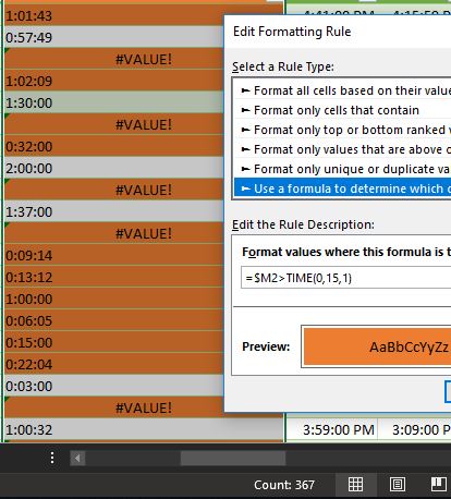
I am trying to write a conditional formatting formula that says anything in column M that is greater than 15 minutes, (0,15,1) should be highlighted. I've tried using the "Format all cells based on their values" and set one for <TIME(0,15,0) and one for >TIME(0,15,1) but that doesn't do anything at all. Same thing with ="TIME(0,15,1)" and ="TIME(23,59,59)" for min/max values
I've also tried =TEXT($B$1,"hh:mm:ss")>"00:15:00" but that highlighted everything in the entire column.
I've tried using the one below but that too doesn't work, it highlights random things but not what I want.
=(M2+0 > TIME(0,15,0))
I tried formatting column M as time hh:mm:ss in cell format, with no real difference. I then tried formatting it as text, and same, no difference. I don't mind if I get a negative value, represented by #VALUE! since I can filter those out.
Colum K Column L Column M
| 3:00:00 PM | 4:01:43 PM | 1:01:43 |
| 1:00:00 PM | 1:57:49 PM | 0:57:49 |
| 10:00:00 AM | 9:02:00 AM | #VALUE! |
| 10:00:00 AM | 11:02:09 AM | 1:02:09 |
| 9:00:00 AM | 10:30:00 AM | 1:30:00 |
| 9:30:00 AM | 9:00:00 AM | #VALUE! |
| 9:00:00 AM | 9:32:00 AM | 0:32:00 |
| 1:00:00 PM | 3:00:00 PM | 2:00:00 |
| 2:00:00 PM | 1:57:34 PM | #VALUE! |
| 10:30:00 AM | 12:07:00 PM | 1:37:00 |
| 10:00:00 AM | 9:04:53 AM | #VALUE! |
| 11:00:00 AM | 11:09:14 AM | 0:09:14 |
| 8:00:00 AM | 8:13:12 AM | 0:13:12 |
| 3:00:00 PM | 4:00:00 PM | 1:00:00 |
| 1:00:00 PM | 1:06:05 PM | 0:06:05 |
| 10:00:00 AM | 10:15:00 AM | 0:15:00 |
| 8:00:00 AM | 8:22:04 AM | 0:22:04 |
| 8:30:00 AM | 8:33:00 AM | 0:03:00 |
| 1:00:00 PM | 12:58:14 PM | #VALUE! |
| 2:00:00 PM | 3:00:32 PM | 1:00:32 |
| 2:15:00 PM | #VALUE! | |
| 11:30:00 AM | 11:35:00 AM | 0:05:00 |
| 10:30:00 AM | 10:10:00 AM | #VALUE! |
| 1:00:00 PM | 1:06:00 PM | 0:06:00 |
| 2:30:00 PM | 2:54:00 PM | 0:24:00 |
| 2:30:00 PM | 1:15:00 PM | #VALUE! |
| 10:00:00 AM | 10:16:36 AM | 0:16:36 |
| 11:00:00 AM | 10:49:00 AM | #VALUE! |
| 8:30:00 AM | 8:55:00 AM | 0:25:00 |
| 1:00:00 PM | 1:15:00 PM | 0:15:00 |
| 3:25:00 PM | 4:10:00 PM | 0:45:00 |
| 10:00:00 AM | 10:50:57 AM | 0:50:57 |
| 3:25:00 PM | 4:10:00 PM | 0:45:00 |
| 10:00:00 AM | 10:25:08 AM | 0:25:08 |
| 11:00:00 AM | 11:25:00 AM | 0:25:00 |
6 Replies
It appears to work - see the screenshot and attached workbook.
If you can't get it to work, could you attach a copy of your workbook without sensitive/proprietary information?
 Steve_BaroneCopper ContributorThanks, I attached a bit of the data in my other reply, with all sensitivity removed.
The formula in C2 should be =B2-A2, not =TEXT(...).
And your conditional formatting formula should not refer to M2 in this sample workbook but to C2, of course.
But it's easier to use a rule of the type "Format only cells that contain".
- SergeiBaklanDiamond Contributor
That's like
In formula it shall be reference on first cell in the range if that's not M1.
In future please submit small sample file instead of / in addition to copy/pasted as text range.
- Steve_BaroneCopper Contributor
I attached a sample of my data, I am using Office 2016.
When I tried it, it wouldn't work the way it did for you. Does it matter that I factored in headers? I made it M2 instead of M1. Not sure if my picture that I tried to upload worked, I can't see it again.
- SergeiBaklanDiamond Contributor
Another option compare to what HansVogelaar suggested is keep the range to which conditional formatting is applied as it is, i.e. entire column C. I'm not sure why you convert time difference into the text, but we also could keep it as it is.
With that we may apply the rule as
using absolute references on Start/End columns and relative reference on current row, starting from very first row of the range, i.e. first one.
With that it doesn't matter which information you return into column C, we only format it depends on values in Time and Actual Time columns.
Bottom line - creating formula for the rule always do it for the first cell of the range to which the rule is applied and take care about absolute/relative references to be sure formula correctly works if virtually move it on another cells.