Forum Discussion
Same Formula, Same Input, Different Results - VLOOKUP with nested IF referencing two columns
The result is a #REF! error.
I can kind of understand what your formula is saying, but I'll read up on INDEX, MATCH and SUMPRODUCT to get a better idea. I hadn't considered those types of formulas.
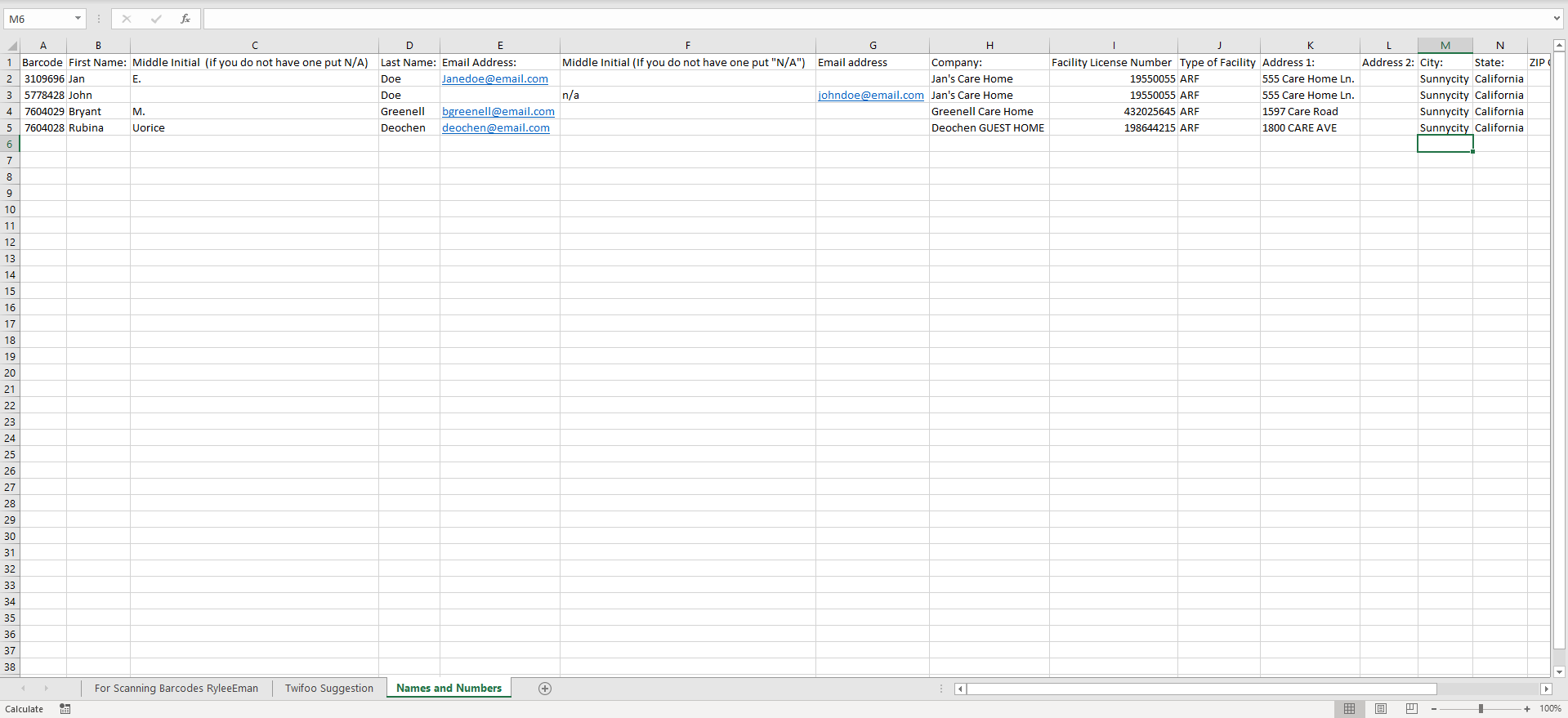
=IF(B2="","",
INDEX(('Names and Numbers'!$C$2:$C$999,'Names and Numbers'!$F$2:$F$999),
MATCH(B2,'Names and Numbers'!$A$2:$A$999,0),1,
SUMPRODUCT(1+('Names and Numbers'!$C$2:$C$999=""))))
I bet that the foregoing formula is faster than 2 IF-VLOOKUPs. If there is an additional Lookup Column, such column has to be added to the reference argument of INDEX and another comparative array has to be added to the array1 argument of SUMPRODUCT.
Conversely, another IF-VLOOKUP combination would have to be added, if the VLOOKUP formula would be used instead of the elegant reference form of INDEX.
 RyleeEmanMar 22, 2019Copper Contributor
Thank you very much for trying to help me
The formula you suggested still gives results in #REF! .
However, I'll keep looking into INDEX and MATCH, since Microsoft Excel also recommends using them for more specific complex formulas needs versus VLOOKUP which seems more basic. I'll probably need it for another formula that will be taking the times inputted when people scan their barcodes, and organize a clean time in and time out on another sheet.
However, the solution for this issue (if C is empty, the use F, otherwise use C) can still be achieved using VLOOKUP and IF; I posted it in this conversation yesterday.