Copying Conditional formatting with relative cell referencces in the formula desn't work

Carsten2900 , you are welcome.

That's quite old discussion, not sure which exactly formula do you mean. In general conditional formatting rule formula iterates cells in the range, to which the rule is applied, the same way as the same formula in the grid (outside your range) which you is entered against first cell of the range and after that dragged right and down.

SergeiBaklan  I don't get the logic in this rule, but it works fine and solved an issue regarding formatting cells with relative reference! Thanks!

BoWan 

Dear, thanks for taking your time to exactly trace out the errors in the formula.  This formula actually works as planned but the relative reference doesn't change the cell reference by copying down our recipe. I think there is a glitch which we aren't able to catch, due to which this happens. 😉

If at any time you're able to achieve the same with relative reference changing on the given cell, Kindly share the same.

Thanks once again.

SergeiBaklan 

Hi, thanks for your advice, but it does NOT work. I have followed your instructions exactly, but NO new rules are created when I step through all cellls in the range with the mouse button. There is only the original rule, but the "Applied to" is just expanded and refers to the same compared cell as in the first rule.

Morisn 

Hi, Bonjour!

Dear Oscar,

Hope your are doing well,  as I opened my outlook today, read your e-mail concern and quickly started to trial the formula that you have put forward.  As I had similar concern last year and got some help here and some formula just worked, just by changing values here and there.

So here is your formula that you need to modify a little bit to get what you need to do in M.S Excel.

Formula: =NOT(ISBLANK($A2)) Format: Amber Applies to: =$B$2:$F$2,$B$2:$F$300

The difference here is that we are applying formula to cell reference only and format to whole table array.

This formula does the intended work as a result.

Just apply conditional formatting to one of the cell and copy that cell up to ranges you're applying to.

Here is the formula snapshot.

https://paste.pics/IU8M3

Hope this works for you and get the most out of M.S Excel.

Thanks & Regards

Hamad B

Hello there,

Since I don't know if this thread is still alive, I'll be very brief. I am having a similar problem with formatting but what I want to achieve is the following:

Simply, every time that I enter 'Y' on Column A, I want the entire row to change colour. As simple as that.

Actually, I don't even care if it's Y or Nay, as long as that row changes colour when it's not blank. Since I am not allowed to add images in this thread, I am sending the Gyazo link where I captured the examples I want to show.

But first, the formula.

I created a rule first, for row no. 2 as follows:

Formula: =NOT(ISBLANK($A$2)) Format: Amber Applies to: =$B$2:$E$2

When trying to figure out how to replicate, the only way I was able to do it the way I wanted was to duplicate the formula and change its values manually. 

I did that 6 times before I got tired.

The rows I added and modified can be seen here:

https://gyazo.com/2fbd83b871a38ddccba5f01f044362e9

And a sample of the results:

First date row (2) with a 'Y' changes row no. 2 colour to amber:

https://gyazo.com/1c8fce73dee70e8397c6ec161406d6ca

And another one:

https://gyazo.com/23e82b0e0bdd83e82dbde7dceee2edcf

Now, for a few rows, it's doable; however, this is completely impractical and backwards for software such as Excel to be doing this for any number of rows. So there should be a better way to do this.

I have about 300 records to apply this to and may be more.

Hopefully, someone could give me an idea of how to go about this.
Thank you and regards,
Oscar

krozar 

Thank you so much for explaining that you have to remove the second "$" to get the relative value for each cell!!

StevanMuller12 

Rule formula could be like =$B2<>$C2 applied to entire range as B2:C999.

With sample file which shows the same data as on screenshot it'll be easier to demonstrate.

Good Day,

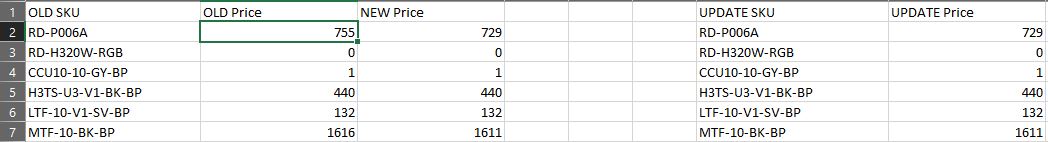
We are trying to show the difference in price change of 2 lists of sku and prices.
And original conditional formatting does not have a rule for this help will be much appreciated.

Jbetteridge91435 , glad to help

SergeiBaklanThankyou very much. this has saved me sooooo much time!! your the real MVP!! 

AaronWalker 

Yes, but first one could have side effect in some situations

SergeiBaklan 

Yes, looks like both methods will work provided that the first row of data is selected in the current section.  All good!  Thanks for sharing.

AaronWalker 

Please check in Sheet2 attached

SergeiBaklan 

What you are showing in your reply will not work.  However, the format I presented works for me in my workbook which was attached.  Since I am new to this, I am not sure you see it.  Anyway, good luck.

AaronWalker 

In general

=D11<>C11     Red
=D11=C11     Green

will be more correct

krozar 

Two Rules:  formulas

=D11:D15<>C11:C15     Red

=D11:D15=C11:C15     Green

Applies to: =D11:D15<>C11:C15     same in both rules

SergeiBaklan 

Thank you for calling out the one subtle difference that allows the format painter to retain relative references!

For those still confused, notice the differences to the rule cell values as shown below:

Original Rules

New Rules

Changing $A$1 to $A1 allowed the format painter to paste relative values to rest of the cells.

Thanks for you your help SergeiBaklan 

krozar 

It shall be relative reference for the row, e.g. Cell Value = $A1. Otherwise you always compare with the value in A1.

Okay, I'm trying these methods, and it's not working for me.  In my case, I have 2 columns with values, A and B.  Column A contains fixed values.  Column B has values either entered manually, or from a formula.

Example:

For cell B1, I have the following two conditional formats applied:

So I'm chaging the text color of B1 to green when the value matches A1, or red if it doesn't match.

I need to copy both formatting rules to the rest of column B, with each cell referencing it's A column counterpart.  Example of how it should look:

None of the formatting copy methods I've tried are working.  Each one is retaining the original A1 cell value comparison.

Am I missing something, or have I overlooked a step?

SergeiBaklan - thanks for this, i've had the same issue this week- trying to copy conditional format to hundreds of cells but needing the reference cell to change each time also. 

the answer above of double click and then using arrows resolved this for me. thank you!