pivottable
27 Topics
Pivot Table grouping defaults to Month when I add data to data source
I have a Pivot Table which is grouped by Year. When I add new records to data source, then hit refresh in Pivot Table, the grouping defaults to Month. I would like it to remain by Year. I tried the 'Disable automatic grouping of Date/Time columns in PivotTables' but that did not work. Any suggestions? Thank you,Solved3.8KViews0likes3Comments
PivotTable : Unexpected behavior with 2 tables
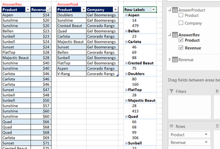
Hi, The first picture shows the expected behavior of adding 'Product' and 'Revenue' to a pivot table. Now when i add the same fields but from 2 different tables linked with a relationship, the result is different (please see 2nd picture). Could somebody explain this weird behavior ? Thanks in advance PivotTable with 1 table PivotTable with 2 tables RelationshipSolved1.8KViews0likes2Comments
Unable to edit calculate values in a PivotTable
I have a pivot table, created by my colleague; it includes calculated values, and I am unable to see its formulas. The following steps were taken: 1) select cell in the pivot table; 2) click "Fields, Items & Sets" ( "PivotTable Analysis" on the ribbon); 3) choose "Calculated Field." Here I expect to see existing calculating fields in the "Name" drop-down list. DD list is empty. As a workaround, I take a look at another excel-file with those values (excel-university.com/edit-pivottable-values) but faced the same problem.3.1KViews0likes3CommentsExcel Update Pivot Table Source Not Working
Folks, I'm adding Pivot table source update comment in case others have the same problem. Problem I created a pivot table whose source data changed because I added rows to the source. When I clicked on the Change Source Button to extend the pivot table source to the additional rows, the Change PivotTable Source window popped up, but Excel did not return to the source data tab with the current row and columns marked. Instead, it just remained on the Pivot table tab. When I manually entered the new table source rows and columns on the Change PivotTable Source form and clicked ok, Excel erased my Pivot table. Normal Operation Excel is supposed to take you to the source table tab with the current selection marked, where you can either mark the new source rows and columns with your mouse or manually enter the rows and columns. When you press Ok on the Change PivotTable Source pop-up, Excel is supposed to update your Pivot table with information from the new source rows and columns. Solution Navigate to the Excel Options’ Data tab and uncheck “Prefer the Excel Data Model when creating PivotTables, QueryTables and Data Conversions.” If you need to leave this option checked, be careful to uncheck Add this data to the Data Model on the Create PivotTable pop-up when creating a new Pivot table.6.1KViews0likes1CommentPivotTable - Calculated Field Subtotal
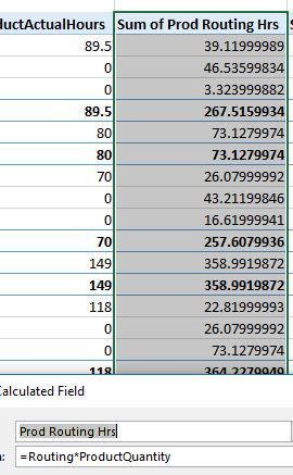
I inserted in a calculated field into a pivot table that multiplies 2 values (this field is titled "sum of Prod Routing Hrs" in the table (see screenshot) and the automatic subtotal on the date (in the row field) will also multiply the values instead of sum them like it does for the other values. Any ideas on how I can fix this? I have also included a screenshot of the calculated field.2.1KViews0likes1CommentSCENARIO PIVOT TABLE
Hi everyone, I am really having difficulty understanding what the following steps are sking me to do. The current chart I have is not what I am supposed to be getting. Any help is appreciated please! Thank you!! Switch back to the All Products Use the Scenario Manager as follows to compare the profit per unit in each scenario: Create a Scenario PivotTable report for result cells B17:D17. Remove the Filter field from the PivotTable. Change the number format of the Profit_per_Unit_Sold_Single_Cup, Profit_per_Unit_Sold_Auto_Drip, and Profit_per_Unit_Sold_French_Pre fields (located in the Values box of the PivotTable Field List) to Currency with 2 decimal places and $ as the symbol. Use Single Cup as the row label value in cell B3, Auto Drip as the value in cell C3, and French Press as the value in cell D3. In cell A1, use Profit per Unit Sold as the report title. Format the report title using the Title cell style. Resize column A using AutoFit. Resize columns B-D to 00.12KViews0likes0Comments
Pivot Table: Two-way Show Values As:
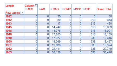
The PivotTable shown below is based on installed pipe length source data in a separate tab. The PivotTable sums those lengths and shows them as running totals by year (row) for each material (column). This shows the cumulative amount of any material installed up to the year on that row. For example: Up to 1943, there had accumulated 117 ft of pipe material "CAS" installed. 30 ft in 1922, 0 ft in 1942, 87 ft in 1943 (30+0+87=117) Now: I want to compute the percentage each cumulative total is of the grand total. So, the 117 ft then formed 27% of the cumulative system total (430 ft) installed up through 1943. Implemented on the whole PivotTable this would show how the composition of the system changed over time. I don't see a way to automate that second computation as a PivotTable feature. I have fallen back on a manual "table" to the right of the PivotTable divides each cumulative value by the value in the Grand Total column on that row. Is there an automated way to do that instead? Or perhaps a better work around?2.5KViews0likes3CommentsPivot Table formatting after refresh
I have a pivot table set up, and have selected "Preserve cell formatting on update" in PivotTable Option. However, when I select a different slicer or refresh the data, the cell formats change dramatically and seemingly randomly. I cannot get the table to save the cell format consistently. Extremely frustrating, and a seemingly known issue with no good fix. Help!!!104KViews3likes26Comments
Pivot table displaying percentage
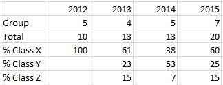
How can I get the following output using pivot table or any other way: I am able to get Group and total but unable to get the %. The % scenario is, if 2012 has all X then it is 100%. Likewise following years have their respective X, Y and Z percentage which has to be calculated and display as in the above picture.675Views0likes0Comments
Percentage calculation in pivot table for a growing time series
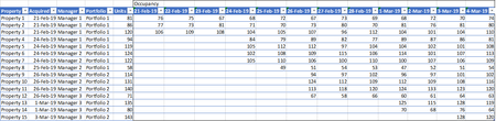
Howdy, I'm trying to create a pivot table showing percentage occupancy across a portfolio of residential properties. The viewer should have the ability to slice the data however they want. I'm unsure how to accomplish this. The basic idea and issues are as follows: Everyday we get an update on the occupancy across the portfolio Some of the properties were added over time so the total number of units has changed multiple times I want to create a pivot table and pivot chart that grow daily to accommodate the newly reported occupancy. The pivot chart and table should show occupancy percentage which are calculated by dividing the occupancy for the period by the number of units during the period. Since I can't add percentages, I'm struggling to figure out how to accomplish this. I want to eventually post the pivot chart with the slicing functionality to a sharepoint site Here is an example of the data. Everyday there will be another column added. Properties start showing occupancy from the day they are acquired. Thanks, elansr1.1KViews0likes0Comments