performance
61 TopicsGeneric Best Practices for HikariCP with Azure Database for PostgreSQL
Author: Mohamed Baioumy Technology: Azure Database for PostgreSQL (Flexible Server & Single Server) Category: Connectivity | Performance | Application Design Introduction Connection pooling is a critical component of application performance when connecting to Azure Database for PostgreSQL. Creating a new PostgreSQL connection is an expensive operation that consumes CPU, memory, and networking resources. Reusing existing connections through a connection pool significantly reduces connection latency, improves throughput, and helps applications scale more efficiently. Many Java applications use HikariCP, one of the most popular high-performance JDBC connection pools. While HikariCP provides excellent performance out of the box, improperly configured connection pool settings can lead to issues such as: Connection pool exhaustion Stale or invalid connections Increased connection acquisition latency Excessive connection creation and destruction Database resource contention Application timeouts This article summarizes generic guidance and best practices for configuring HikariCP when working with Azure Database for PostgreSQL Flexible Server and Azure Database for PostgreSQL Single Server. Understanding Key HikariCP Parameters 1. Maximum Lifetime (maxLifetime) The maxLifetime property controls how long a connection can remain in the pool before HikariCP retires it and creates a new one. Why It Matters Connections can become stale over time due to: Network interruptions Infrastructure updates Connection state changes TCP idle behavior Recycling connections periodically helps prevent applications from using long-lived connections that may no longer be healthy. Recommended Practice Avoid configuring the value too low. When maxLifetime is set aggressively, HikariCP continuously destroys and recreates connections, resulting in: Additional authentication overhead Increased connection establishment latency Higher CPU utilization Reduced application throughput A reasonable starting point is: spring.datasource.hikari.maxLifetime=1800000 30 minutes (1,800,000 ms) is commonly used and aligns well with many production workloads. Depending on workload characteristics, values between 30 minutes and 1 hour are generally suitable Avoid maxLifetime=300000 (5 minutes) This often causes unnecessary connection churn without providing additional benefits. 2. Minimum Idle Connections (minimumIdle) The minimumIdle setting defines how many idle connections HikariCP should keep ready for immediate use. Why It Matters A pool with available idle connections can serve application requests immediately without waiting for new connections to be established. However, maintaining too many idle connections consumes unnecessary database resources. Recommended Practice For most workloads: minimumIdle = maximumPoolSize Or minimumIdle slightly lower than maximumPoolSize This ensures sufficient connections are already available during traffic spikes while avoiding excessive connection creation delays. Example maximumPoolSize=20 minimumIdle=15 Avoid maximumPoolSize=20 minimumIdle=20 only when the application experiences long periods of inactivity and conserving resources is more important than immediate responsiveness. 3. Idle Timeout (idleTimeout) The idleTimeout property determines how long an unused connection remains in the pool before being removed. Why It Matters Connections that sit idle for extended periods consume resources on both: The application server Azure Database for PostgreSQL However, removing idle connections too quickly causes the application to repeatedly establish new connections. Recommended Practice Keep the default value unless there is a specific requirement. spring.datasource.hikari.idleTimeout=600000 which equals: 10 minutes (600,000 ms) This setting provides a good balance between resource utilization and responsiveness. [Re: EXT: R...0040002947 | Outlook] The timeout should also be comfortably longer than any expected short application idle periods. Avoid idleTimeout=10000 (10 seconds) Such aggressive settings often result in unnecessary connection creation cycles. 4. Maximum Pool Size (maximumPoolSize) This parameter determines the maximum number of concurrent database connections the application can maintain. Why It Matters This is often the most important HikariCP setting. If the Pool Is Too Small Applications may experience: Connection is not available, request timed out because all available connections are already in use. Similar scenarios have been observed during customer investigations involving Hikari pool exhaustion. If the Pool Is Too Large Applications can overwhelm the database server with excessive concurrent sessions, resulting in: Connection contention Increased context switching Higher memory consumption Reduced overall performance Recommended Practice Pool size should be based on: Database compute configuration CPU core count Query execution duration Application concurrency requirements Workload characteristics There is no universal value that fits every workload. Start conservatively: maximumPoolSize=10 or maximumPoolSize=20 maximumPoolSize=20 and increase only after load testing demonstrates a need for additional concurrency. Fixed-Size Pool Recommendation For many production workloads, a fixed-size pool provides the simplest and most predictable behavior. Configure: maximumPoolSize=20 minimumIdle=20 or omit minimumIdle entirely so it defaults to maximumPoolSize. HikariCP commonly recommends maintaining a fixed-size pool for responsiveness during demand spikes. Benefits Faster connection acquisition Predictable performance Reduced connection creation latency Better handling of traffic spikes When using a small fixed-size pool, there is often little need to aggressively tune: minimumIdle idleTimeout Instead, simply recycle connections using: maxLifetime maxLifetime Additional Recommendations Enable TCP Keepalive One common cause of stale connections is network devices silently dropping inactive TCP sessions. For PostgreSQL applications, consider enabling TCP keepalive: tcpKeepAlive=true tcpKeepAlive=true The HikariCP project specifically recommends enabling TCP keepalive to prevent rare situations where pools can lose valid connections. Monitor Connection Usage Track: Active connections Idle connections Connection acquisition time Pool exhaustion events Database connection counts These metrics help identify whether pool sizing is appropriate. Investigate Long-Running Queries Connection pool problems are often symptoms rather than root causes. A frequent scenario is: A query becomes slow. Connections remain occupied longer. The pool becomes exhausted. Applications start timing out. When analyzing HikariCP issues, always review: Query performance Blocking situations Database resource utilization Application connection handling logic Sample Production Configuration spring.datasource.hikari.maximumPoolSize=20 spring.datasource.hikari.minimumIdle=15 spring.datasource.hikari.maxLifetime=1800000 spring.datasource.hikari.idleTimeout=600000 spring.datasource.hikari.connectionTimeout=30000 spring.datasource.hikari.keepaliveTime=60000 spring.datasource.hikari.maximumPoolSize=20 spring.datasource.hikari.minimumIdle=15 spring.datasource.hikari.maxLifetime=1800000 spring.datasource.hikari.idleTimeout=600000 spring.datasource.hikari.connectionTimeout=30000 spring.datasource.hikari.keepaliveTime=60000 This configuration provides a solid starting point for many Azure Database for PostgreSQL workloads and can be adjusted based on application-specific requirements. a { text-decoration: none; color: #464feb; } tr th, tr td { border: 1px solid #e6e6e6; } tr th { background-color: #f5f5f5; } Conclusion HikariCP is extremely efficient when configured appropriately. The goal is not to maximize the number of connections, but rather to maintain a healthy balance between application responsiveness and database resource consumption. As a general rule: Use a reasonable maxLifetime (30–60 minutes) Keep enough idle connections available for traffic spikes Avoid aggressive idleTimeout values Size the pool based on workload characteristics, not guesses Consider fixed-size pools for predictable performance Monitor connection usage and query performance regularly By following these practices, applications connecting to Azure Database for PostgreSQL can achieve improved scalability, lower latency, and more reliable connectivity. References Connection pooling best practices - Azure Database for PostgreSQL Performance best practices for using Azure Database for PostgreSQL – Connection Pooling HikariCP Documentation and Pool Sizing GuidanceLessons Learned #540:Bulk Insert Throughput in Azure SQL Hyperscale with Partitioned Heap Tables
In this lesson learned, I would like to share an interesting scenario working on a service request where our customer was running a high-volume data load process in Azure SQL Database Hyperscale. The workload was based on a common pattern: Recreate a staging table. Load a large number of rows using bulk insert. The bulk insert showed unstable execution times and became the main area to investigate. The process was loading a very large number of rows into an Azure SQL Database Hyperscale database. The process used a staging table that was initially loaded as a heap. The main concern was the inconsistent execution time during the load process. Why Manually Adding Data Files Was Not the Right Direction In Azure SQL Database Hyperscale, the storage architecture is different from a traditional SQL Server deployment. The data layout and storage management are handled internally by the service. Because of this architecture, manually creating or pre-allocating multiple data files is not the same tuning option that we may consider in SQL Server on-premises or SQL Server running on Azure Virtual Machines. For this reason, the troubleshooting focus moved from manual file layout configuration to the actual workload pattern, waits, concurrency, batch size, and staging table design. What We Observed During the bulk insert phase, waits such as PAGELATCH_EX were observed. Since the staging table was loaded as a heap and the clustered primary key was created only after the bulk insert completed, OPTIMIZE_FOR_SEQUENTIAL_KEY was not directly applicable to the bulk insert phase. This changed the direction of the investigation. Instead of focusing on last-page insert contention on an existing clustered index, the analysis moved toward heap insert behavior, allocation contention, concurrency, batch size, and whether a different staging table design could help. First Recommendation: Start with Low-Impact Changes Before changing the table design, the first recommendation was to test the least intrusive changes: Reduce the number of concurrent bulk insert sessions. Increase the batch size, for example from 10,000 rows to 50,000 or 100,000 rows. Test TABLOCK on the dedicated heap staging table. The goal was to avoid assuming that more concurrency would always reduce the total execution time. In some high-volume load scenarios, excessive concurrency may increase contention and make the process less stable. The Interesting Design Option: Partitioned Heap Staging Table One of the most interesting design options was to evaluate a partitioned heap staging table. The idea is simple: instead of loading all rows into a non-partitioned heap staging table, the staging table can be created on the same partition scheme used by the target table, using the same partitioning column. This does not mean that a partitioned heap will always be faster. However, it can be a useful design option when: The bulk load phase is affected by allocation or latch contention. Concurrent load processes can naturally distribute rows across different partition ranges. The staging table is used only as an intermediate structure.Lessons Learned The main lessons from this scenario were: In Azure SQL Database Hyperscale, manually managing multiple data files is not the right tuning direction. PAGELATCH_EX during heap loading may point to concurrency or allocation-related contention. Reducing concurrency can sometimes improve total throughput. Larger batch sizes may provide better results than many small batches. TABLOCK on a dedicated heap staging table is a low-impact test worth evaluating. A partitioned heap staging table can be a valid second-phase design option when the load can be distributed across partition ranges. The best approach is to test small, measurable changes before introducing architectural redesigns. Final Thoughts A partitioned heap staging table can be a powerful option, but only when it is tested carefully and when the workload pattern can benefit from partition distribution.251Views0likes0CommentsLessons Learned #547:Some SQL DB Statistics Remain Outdated While Others Are Automatically Updated
During the analysis of a SQL Server performance case, we observed an interesting statistics update pattern on a large table. Several statistics had recently been updated at different times, while a group of automatically created _WA_Sys_ statistics still showed: An older last_updated date. A high modification_counter. A row count significantly lower than the current number of rows in the table. At first glance, this could suggest that AUTO_UPDATE_STATISTICS was not working correctly. However, a closer review showed that this pattern can be completely consistent with the expected behavior of SQL Server. 1. Types of statistics in SQL Server SQL Server can maintain several types of statistics. Automatically created column statistics When AUTO_CREATE_STATISTICS is enabled, SQL Server can automatically create a single-column statistic when the Query Optimizer needs cardinality information for a column used in a query predicate. These statistics normally use names such as: _WA_Sys_00000002_47A6D5E5 The name can be interpreted as: _WA_Sys_<column_id in hexadecimal>_<object_id in hexadecimal> For example: 00000002 hexadecimal = column_id 2 47A6D5E5 hexadecimal = table object_id The most reliable way to identify the associated column is not to decode the name manually, but to query the SQL Server catalog views: DECLARE @TableName sysname = N'dbo.CustomerTransactions'; SELECT s.stats_id, s.name AS statistics_name, sc.stats_column_id, c.column_id, c.name AS column_name, s.auto_created, s.user_created, s.no_recompute FROM sys.stats AS s INNER JOIN sys.stats_columns AS sc ON sc.object_id = s.object_id AND sc.stats_id = s.stats_id INNER JOIN sys.columns AS c ON c.object_id = sc.object_id AND c.column_id = sc.column_id WHERE s.object_id = OBJECT_ID(@TableName) AND s.name = N'_WA_Sys_00000002_47A6D5E5' ORDER BY sc.stats_column_id; Statistics associated with indexes When SQL Server creates an index, it also creates a statistics object associated with the index. For example: CREATE INDEX IX_CustomerTransactions_ClientId ON dbo.CustomerTransactions(ClientId) this creates an index statistics object normally named: IX_CustomerTransactions_ClientId when a statistics object corresponds to an index, its stats_id matches the index's index_id. User-created statistics Statistics can also be created explicitly: CREATE STATISTICS ST_CustomerTransactions_ClientId_Status ON dbo.CustomerTransactions ( ClientId, StatusId ); This object is identified in sys.stats with: user_created = 1 auto_created = 0 and AUTO_UPDATE_STATISTICS applies to index statistics, automatically created single-column statistics, manually created statistics and filtered statistics. 2. Statistics are not updated together Assume that a table has these statistics: _WA_Sys_00000002_xxxxxxxx for ClientId _WA_Sys_00000003_xxxxxxxx for StatusId IX_CustomerTransactions_CreatedDate for CreatedDate PK_CustomerTransactions and TransactionId After a large data load, several or all of them could become eligible for an automatic update. However, SQL Server does not immediately update all eligible statistics. Before compiling a query, the Query Optimizer identifies the statistics that could be relevant to the query predicates and checks whether those statistics are outdated. Consider this query: SELECT TransactionId, ClientId, Amount FROM dbo.CustomerTransactions WHERE ClientId = 100; The optimizer might need a histogram on ClientId. If the corresponding statistics object is outdated and has crossed its update threshold, SQL Server may update that specific statistics object. It does not need to update unrelated statistics on: StatusId CreatedDate As a result, statistics on the same table can legitimately have different update times: PK_CustomerTransactions 2026-07-22 10:53 IX_CustomerTransactions_ClientId 2026-07-22 10:50 IX_CustomerTransactions_CreatedDate 2026-07-22 10:13 _WA_Sys_00000003_47A6D5E5 2026-07-19 10:00 This pattern can be evidence of demand-driven automatic updates rather than evidence of a malfunction. 3. What does modification_counter represent? The modification_counter returned by sys.dm_db_stats_properties represents the number of modifications made to the leading statistics column since that statistics object was last updated. This definition is especially important for multicolumn statistics. For example: CREATE INDEX IX_CustomerTransactions_ClientId_Status ON dbo.CustomerTransactions ( ClientId, StatusId ); The associated statistics object contains: Histogram: ClientId Density information: ClientId ClientId, StatusId The histogram and modification_counter are based on the leading column, ClientId. If only StatusId is modified: UPDATE dbo.CustomerTransactions SET StatusId = 2 WHERE TransactionId = 100; this does not have the same statistics impact as changing ClientId, because ClientId is the leading histogram column. SQL Server statistics contain only one histogram, built on the first key column. Multicolumn statistics additionally contain density information for column prefixes. 4. Why do multiple statistics sometimes have similar modification counters? This commonly happens after an insert operation. For example: INSERT INTO dbo.CustomerTransactions ( TransactionId, ClientId, StatusId, Amount, CreatedDate ) SELECT TransactionId, ClientId, StatusId, Amount, CreatedDate FROM dbo.StagingCustomerTransactions; Each inserted row introduces a value for every populated column. Consequently, multiple single-column statistics may show similar increases in their modification counters. This is particularly visible after a large ETL operation: Table rows before the load: 487,673 Rows inserted by the ETL: 515,244 Current approximate row count: 1,002,917 Several statistics could then show modification counters close to the number of inserted rows. That does not mean SQL Server must update all those statistics immediately. They become candidates for updating, but an update is normally triggered when query optimization requires them. 5. Does automatic updating apply only to _WA_Sys_ statistics? AUTO_UPDATE_STATISTICS applies to: Automatically created _WA_Sys statistics Index statistics Primary-key index statistics User-created statistics Each statistics object is evaluated independently. Therefore, SQL Server might update: PK_CustomerTransactions while leaving this object unchanged: _WA_Sys_00000003_47A6D5E5 The reverse is also possible. The behavior depends on which statistics are considered relevant during compilation or cached-plan validation. 6. What happens when a _WA_Sys_ statistic and an index statistic cover the same column? This is one of the most interesting scenarios. Assume SQL Server originally created: _WA_Sys_00000002_xxxxxxxx for ClientId. Later, someone creates this index: CREATE INDEX IX_CustomerTransactions_ClientId ON dbo.CustomerTransactions(ClientId); The table now has two statistics objects with histograms on ClientId: _WA_Sys_00000002_xxxxxxxx and IX_CustomerTransactions_ClientId Conceptually: _WA_Sys statistic Histogram on ClientId Index statistic Histogram on ClientId For a query such as: SELECT * FROM dbo.CustomerTransactions WHERE ClientId = @ClientId; the optimizer can have more than one potentially relevant statistics object. It may rely on the index statistics object rather than the older _WA_Sys_ object. In that case: IX_CustomerTransactions_ClientId Updated recently _WA_Sys_00000002_xxxxxxxx Old last_updated value High modification_counter This does not necessarily mean that automatic statistics updating has failed. It can mean that the _WA_Sys_ statistic has become redundant and has not been required by recent compilations. However, this should be presented carefully: The Query Optimizer is not publicly documented as always preferring an index statistic over an equivalent _WA_Sys_ statistic. The statistics selected can depend on: Query. Predicates. Available indexes. Filtered versus unfiltered statistics. Statistics freshness. Sampling quality. Multicolumn density information. Cardinality Estimator behavior. Existing cached plans. The correct conclusion is that the scenario is possible and plausible, but the execution plan should be inspected before claiming that a specific statistics object was used. As we wrote down in multiple articles in our blog (below), identify redudant statistics is part of DBA work to avoid this situation, also, in other situations, I saw that the maintenance plan is taking too much time because we are updating statistics that we are not using or migth be duplicated. The following script identifies statistics whose leading columns overlap: DECLARE @TableName sysname = N'dbo.CustomerTransactions'; ;WITH LeadingStatisticsColumns AS ( SELECT s.object_id, s.stats_id, s.name AS statistics_name, s.auto_created, s.user_created, s.no_recompute, s.has_filter, s.filter_definition, sc.column_id, c.name AS leading_column, i.index_id, i.name AS index_name FROM sys.stats AS s INNER JOIN sys.stats_columns AS sc ON sc.object_id = s.object_id AND sc.stats_id = s.stats_id AND sc.stats_column_id = 1 INNER JOIN sys.columns AS c ON c.object_id = sc.object_id AND c.column_id = sc.column_id LEFT JOIN sys.indexes AS i ON i.object_id = s.object_id AND i.index_id = s.stats_id WHERE s.object_id = OBJECT_ID(@TableName) ) SELECT leading_column, statistics_name, CASE WHEN index_id IS NOT NULL THEN N'INDEX STATISTICS' WHEN auto_created = 1 THEN N'AUTO-CREATED _WA_SYS' WHEN user_created = 1 THEN N'USER-CREATED STATISTICS' ELSE N'OTHER' END AS statistics_type, index_name, has_filter, filter_definition, no_recompute, COUNT(*) OVER ( PARTITION BY column_id ) AS statistics_on_same_leading_column FROM LeadingStatisticsColumns ORDER BY leading_column, statistics_type, statistics_name; This does not automatically mean that one object should be deleted. It only identifies an overlap. 7. Script The following example demonstrates how an automatically created statistic can coexist with a later index statistic. DROP TABLE IF EXISTS dbo.CustomerTransactions; GO CREATE TABLE dbo.CustomerTransactions ( TransactionId int NOT NULL, ClientId int NOT NULL, StatusId tinyint NOT NULL, Amount decimal(12,2) NOT NULL, CreatedDate datetime2(0) NOT NULL, CONSTRAINT PK_CustomerTransactions PRIMARY KEY CLUSTERED (TransactionId) ); GO Insert sample data ;WITH Numbers AS ( SELECT TOP (200000) ROW_NUMBER() OVER ( ORDER BY (SELECT NULL) ) AS n FROM sys.all_objects AS a CROSS JOIN sys.all_objects AS b ) INSERT INTO dbo.CustomerTransactions ( TransactionId, ClientId, StatusId, Amount, CreatedDate ) SELECT n, n % 5000, n % 5, CONVERT(decimal(12,2), n % 10000), DATEADD ( minute, -(n % 100000), SYSUTCDATETIME() ) FROM Numbers; GO Ensure that automatic statistics creation and updating are enable ALTER DATABASE CURRENT SET AUTO_CREATE_STATISTICS ON; GO ALTER DATABASE CURRENT SET AUTO_UPDATE_STATISTICS ON; GO Trigger automatic statistics creation on ClientId SELECT COUNT_BIG(*) FROM dbo.CustomerTransactions WHERE ClientId = 100 OPTION (RECOMPILE); GO Check the statistics created for ClientId SELECT s.stats_id, s.name AS statistics_name, s.auto_created, s.user_created, c.name AS column_name FROM sys.stats AS s INNER JOIN sys.stats_columns AS sc ON sc.object_id = s.object_id AND sc.stats_id = s.stats_id INNER JOIN sys.columns AS c ON c.object_id = sc.object_id AND c.column_id = sc.column_id WHERE s.object_id = OBJECT_ID(N'dbo.CustomerTransactions') AND c.name = N'ClientId' ORDER BY s.stats_id; Create an index on the same column CREATE INDEX IX_CustomerTransactions_ClientId ON dbo.CustomerTransactions(ClientId); The table can now have: Modify the data significantly UPDATE dbo.CustomerTransactions SET ClientId = ClientId + 10000 WHERE TransactionId <= 100000; Review the counters again SELECT s.name AS statistics_name, sp.last_updated, sp.rows, sp.rows_sampled, sp.modification_counter FROM sys.stats AS s OUTER APPLY sys.dm_db_stats_properties ( s.object_id, s.stats_id ) AS sp WHERE s.object_id = OBJECT_ID(N'dbo.CustomerTransactions') ORDER BY s.stats_id Force a new compilation using ClientId SET STATISTICS XML ON; GO SELECT COUNT_BIG(*) FROM dbo.CustomerTransactions WHERE ClientId = 10100 OPTION (RECOMPILE); GO SET STATISTICS XML OFF; GO After the query, review: The actual execution plan XML. The StatisticsInfo elements. last_updated. modification_counter. The exact object updated is an optimizer decision and can vary by SQL Server version, build, compatibility level and query shape. The test should therefore be used to observe the behavior rather than to assume a fixed preference. Finally, as you could see SQL Server choose _WA_Sys_00000002_151102AD instead of IX_CustomerTransactions_ClientId to update. In some situations, depending on execution plan, SQL Server might choose IX_CustomerTransactions_ClientId to update instead of _WA_Sys_00000002_151102AD and for this reason, doesn't mean that SQL Server is not updating the statistics it is depending that it is choosing one of them that the column is involved. My lessons learned, a statistic can be outdated without being relevant, and it can be relevant without being the only available source of cardinality information. Before interpreting an old last_updated value as an automatic statistics failure, identify the leading column, look for overlapping statistics, inspect the execution plan and determine whether there is a real estimation or performance problem. Articles: Lesson Learned #482: Identifying Potential Duplicate Statistics | Microsoft Community Hub Lesson Learned #324: Query Recompilation in Azure SQL | Microsoft Community Hub Lessons Learned #537: Copilot Prompts for Troubleshooting on Azure SQL Database | Microsoft Community Hub Lesson Learned #498:Understanding the Role of STATMAN in SQL Server and Its Resource Consumption | Microsoft Community Hub Disclaimer: The scripts included in this article are provided for demonstration and educational purposes only. They create a sample table, insert a significant number of rows, create indexes and statistics, modify data, and change automatic statistics settings in the current database. Run the complete demonstration only in a test or non-production environment. Review and adapt the database name, object names, row volume, and statements before execution. The results may vary depending on the SQL Server version, database compatibility level, existing configuration, data distribution, and workload. Always test the scripts in a representative environment before applying any conclusion or change to a production system.326Views0likes0CommentsLessons Learned #544: How to Detect INT Identity Exhaustion Before Inserts Fail.
Recently, I worked on a support case involving an Azure SQL Database table where the customer had reached the maximum value supported by the INT data type. The table used an INT IDENTITY(1,1) column as its primary key. Over time, the generated identity value approached the maximum value supported by INT. Once the available range was exhausted, the application was no longer able to insert new rows. At that point, the column needed to be changed from INT to BIGINT. However, performing this type of migration on a very large table can be a complex and time-consuming operation. The situation is that an INT column uses 4 bytes and supports values from: -2,147,483,648 to: 2,147,483,647. To prevent similar problems in the future, I suggested using the following query to review the current status of all INT IDENTITY columns in the database. The query uses the sys.identity_columns catalog view: SELECT s.name AS SchemaName, t.name AS TableName, c.name AS ColumnName, CONVERT(bigint, c.last_value) AS CurrentIdentityValue, CONVERT(bigint, 2147483647) AS MaximumIntValue, CONVERT(bigint, 2147483647) - ISNULL(CONVERT(bigint, c.last_value), 0) AS RemainingValues, CAST( ISNULL(CONVERT(decimal(20,2), c.last_value), 0) / 2147483647 * 100 AS decimal(6,2) ) AS PercentUsed FROM sys.identity_columns AS c INNER JOIN sys.tables AS t ON c.object_id = t.object_id INNER JOIN sys.schemas AS s ON t.schema_id = s.schema_id WHERE TYPE_NAME(c.system_type_id) = 'int' ORDER BY PercentUsed DESC; I prefer using this query instead of relying on: SELECT COUNT(*) FROM dbo.TableName. The number of rows in a table does not necessarily match the current identity value. Rows might have been deleted, transactions might have been rolled back, and identity values might contain gaps. For this reason, the current identity value is a better indicator of the remaining capacity. Adding this query as a regular preventive check can help identify identity columns that are approaching their limits before they cause application failures. I would like to share with you an example creates a table with an identity seed close to the maximum value supported by INT: DROP TABLE IF EXISTS dbo.IdentityCapacityDemo2; CREATE TABLE dbo.IdentityCapacityDemo2 ( Id INT IDENTITY(2147483600,1) NOT NULL, CreatedDate datetime2(0) NOT NULL CONSTRAINT DF_IdentityCapacityDemo2_CreatedDate DEFAULT SYSUTCDATETIME(), CONSTRAINT PK_IdentityCapacityDemo2 PRIMARY KEY CLUSTERED (Id) ) Insert 20 rows using this command: insert into IdentityCapacityDemo2(CreatedDate) values(SYSUTCDATETIME()) Example of returns: I think runnning this preventive check can help detect identity exhaustion before it affects the application.Lessons Learned #541:Automatic Plan Correction vs External Tables: A Practical Lesson from the Field
Automatic Plan Correction is one of the most useful capabilities in Azure SQL Database when dealing with plan regressions. It uses Query Store to identify when a query starts using a worse execution plan and, when appropriate, forces the last known good plan. However, during a recent troubleshooting scenario, I found that not all queries have the same execution characteristics. In particular, queries that reference external tables may behave differently from fully local queries because part of their execution depends on remote data access. When Query Store is configured to capture all queries, we can use it to identify queries that reference external tables and review whether those query IDs should participate in FORCE_LAST_GOOD_PLAN. From a practical perspective, external-table queries may not always be the best candidates for Automatic Plan Correction, especially when the expected benefit of automatic plan forcing is not clear. For that reason, the goal of this article is simple: identify queries that reference external tables and, when appropriate, exclude selected query IDs from Automatic Plan Correction. If we review the execution plan for the following query: DECLARE @Region nvarchar(50) = N'EMEA' SELECT CustomerId, CustomerName, Region FROM dbo.ExternalCustomers WHERE Region = @Region; We can see that the plan includes a Remote Query operator. This means that the query is not only accessing local data; part of the execution depends on remote data access through the external table. For this type of query, Automatic Plan Correction may not provide the same clear benefit as it does for fully local queries. The performance may depend not only on the local execution plan, but also on the remote database, the external data source, network latency, and the amount of data returned from the remote side. For that reason, queries referencing external tables are good candidates for review before allowing them to participate in FORCE_LAST_GOOD_PLAN. In this scenario, the first step was to identify the Query Store query_id associated with the query referencing the external table. Since the query text was available in Query Store, we searched for the external table name in sys.query_store_query_text. SELECT q.query_id, p.plan_id, p.is_forced_plan, p.plan_forcing_type_desc, p.force_failure_count, p.last_force_failure_reason_desc, p.last_execution_time, qt.query_sql_text FROM sys.query_store_query_text AS qt INNER JOIN sys.query_store_query AS q ON qt.query_text_id = q.query_text_id INNER JOIN sys.query_store_plan AS p ON q.query_id = p.query_id WHERE qt.query_sql_text LIKE N'%ExternalCustomers%' ORDER BY p.last_execution_time DESC; Once the query_id was identified, the next step was to exclude that specific query from Automatic Plan Correction by setting FORCE_LAST_GOOD_PLAN to OFF for that query_id. EXECUTE sys.sp_configure_automatic_tuning @option = 'FORCE_LAST_GOOD_PLAN', @type = 'QUERY', @type_value = N'<query_id>', @option_value = 'OFF'; For example: EXECUTE sys.sp_configure_automatic_tuning @option = 'FORCE_LAST_GOOD_PLAN', @type = 'QUERY', @type_value = N'1574', @option_value = 'OFF'; This does not disable Automatic Plan Correction for the entire database. It only tells Automatic Plan Correction to ignore this specific Query Store query ID for FORCE_LAST_GOOD_PLAN. With this approach, Automatic Plan Correction can remain enabled for the rest of the database workload, while selected queries that depend on external or remote data access can be reviewed and excluded individually when automatic plan forcing is not expected to provide a clear benefit.167Views0likes0Comments
Why do I see many VDI_CLIENT_WORKER sessions in Azure SQL Database — and do they impact performance?
Sometimes you’ll notice many sessions showing the command VDI_CLIENT_WORKER in Azure SQL Database—often around scaling, replica/copy workflows, or internal seeding operations. These sessions can look alarming, especially during a performance investigation, but they are typically internal background workers. This post explains how to recognize them, what’s safe to do (and what isn’t), and how to focus on the real bottlenecks like blocking/deadlocks or log rate throttling when you’re troubleshooting slowness. Why you might see VDI_CLIENT_WORKER sessions in Azure SQL Database The symptom You run a session query (for example, using sys.dm_exec_requests or a monitoring tool) and observe: Many sessions with command text VDI_CLIENT_WORKER They may appear to be “stuck,” persist longer than expected, and can’t be killed Teams may worry these sessions are “the cause” of slowness Why it shows up in Azure SQL In Azure SQL, VDI_CLIENT_* wait types and VDI_CLIENT_WORKER sessions are commonly associated with platform operations that involve copying/seeding—for example: Scaling operations (service objective changes) Geo-replication / copy workflows Replica seeding-like behaviors Important: The presence of these sessions does not automatically mean they are the bottleneck. How to validate whether VDI_CLIENT_WORKER is benign? 1) Correlate to recent platform operations. Ask: did you recently perform (or did the platform perform) one of these? Scale up/down. Creation of replicas / geo-secondary operations. Any database copy-like workflow. If yes, it’s a strong indicator you’re seeing background workers tied to that lifecycle event. 2) Check whether they consume resources. A practical approach: Look for CPU/IO/log pressure at the database level. Compare the timing of slowness reports with spikes in waits/locks/log write percentage. If these sessions show minimal resource consumption and are just “present,” treat them as background noise while you investigate real contention. 3) Don’t try to kill them! These sessions are typically system/internal. Attempts to kill them may fail or be ineffective—and generally aren’t recommended. 4) If you need them to disappear. In many cases, these internal workers naturally age out. If they remain visible and you need a cleanup path, operational actions like failover/restart may clear stale workers (use change control / maintenance windows as appropriate for your environment). (This is a practical operational observation; always weigh downtime/impact.) When performance is actually slow: focus on what usually hurts. In many real-world incidents, the main causes of slowness are: Blocking chains / deadlocks. Transaction log rate throttling (LOG_RATE_GOVERNOR) during heavy DML. Hot queries running concurrently and contending on the same objects. Key takeaways Seeing many VDI_CLIENT_WORKER sessions is often expected around platform copy/seeding workflows and doesn’t automatically indicate a bottleneck. Don’t attempt to kill system/internal workers; instead, validate resource impact and focus on actual bottlenecks. For real slowness, prioritize diagnosing blocking/deadlocks and LOG_RATE_GOVERNOR-driven DML throttling.176Views0likes0CommentsLessons Learned #537: Copilot Prompts for Troubleshooting on Azure SQL Database
We had the opportunity to share our experience in several community sessions how SSMS Copilot can help across multiple phases of troubleshooting. In this article, I would like to share a set of prompts we found in those sessions and show how to apply them to an example query. During a performance incident, we captured the following query, generated by PowerBI. SELECT TOP (1000001) * FROM ( SELECT [t2].[Fiscal Month Label] AS [c38], SUM([t5].[Total Excluding Tax]) AS [a0], SUM([t5].[Total Including Tax]) AS [a1] FROM ( SELECT [$Table].[Sale Key] as [Sale Key], [$Table].[City Key] as [City Key], [$Table].[Customer Key] as [Customer Key], [$Table].[Bill To Customer Key] as [Bill To Customer Key], [$Table].[Stock Item Key] as [Stock Item Key], [$Table].[Invoice Date Key] as [Invoice Date Key], [$Table].[Delivery Date Key] as [Delivery Date Key], [$Table].[Salesperson Key] as [Salesperson Key], [$Table].[WWI Invoice ID] as [WWI Invoice ID], [$Table].[Description] as [Description], [$Table].[Package] as [Package], [$Table].[Quantity] as [Quantity], [$Table].[Unit Price] as [Unit Price], [$Table].[Tax Rate] as [Tax Rate], [$Table].[Total Excluding Tax] as [Total Excluding Tax], [$Table].[Tax Amount] as [Tax Amount], [$Table].[Profit] as [Profit], [$Table].[Total Including Tax] as [Total Including Tax], [$Table].[Total Dry Items] as [Total Dry Items], [$Table].[Total Chiller Items] as [Total Chiller Items], [$Table].[Lineage Key] as [Lineage Key] FROM [Fact].[Sale] as [$Table] ) AS [t5] INNER JOIN ( SELECT [$Table].[Date] as [Date], [$Table].[Day Number] as [Day Number], [$Table].[Day] as [Day], [$Table].[Month] as [Month], [$Table].[Short Month] as [Short Month], [$Table].[Calendar Month Number] as [Calendar Month Number], [$Table].[Calendar Month Label] as [Calendar Month Label], [$Table].[Calendar Year] as [Calendar Year], [$Table].[Calendar Year Label] as [Calendar Year Label], [$Table].[Fiscal Month Number] as [Fiscal Month Number], [$Table].[Fiscal Month Label] as [Fiscal Month Label], [$Table].[Fiscal Year] as [Fiscal Year], [$Table].[Fiscal Year Label] as [Fiscal Year Label], [$Table].[ISO Week Number] as [ISO Week Number] FROM [Dimension].[Date] as [$Table] ) AS [t2] ON [t5].[Delivery Date Key] = [t2].[Date] GROUP BY [t2].[Fiscal Month Label] ) AS [MainTable] WHERE ( NOT([a0] IS NULL) OR NOT([a1] IS NULL) ) I structure the investigation in three areas: Analysis – understand the data model, sizes, and relationships. List all tables in the 'Fact' and 'Dimension' schemas with space usage in MB and number of rows. The name of the tables and their relations among them. Please, provide a textual representation for all relations. List all foreign key relationships between tables in the 'Fact' and 'Dimension' schemas, showing the cardinality and referenced columns. Could you please let me know what is the meaning of every table? Describe all schemas in this database, listing the number of tables and views per schema. Create a textual data model (ER-style) representation showing how all Fact and Dimension tables are connected. Maintenance Plan Check – verify statistics freshness, index health/fragmentation, partition layout, and data quality. List all statistics in the database that have not been updated in the last 7 days, showing table name, number of rows, and last update date. List all indexes in the database with fragmentation higher than 30%, including table name, index name, and page count. Please, provide the T-SQL to rebuild all indexes in ONLINE mode and UPDATE STATISTICS for all tables that are automatic statistics. Check for fact table rows that reference dimension keys which no longer exist (broken foreign key integrity). Find queries that perform table scans on large tables where no indexes are used, based on recent execution plans. Performance Improvements – simplify/reshape the query and consider indexed views, columnstore, partitioning, and missing indexes. In this part, I would like to spend more time about these prompts, for example the following ones, help me to understand the performance issue, simplify the query text and also, explains what the query is doing. Identify the longest-running query in the last 24 hours provide the full text of the query Please simplify the query Explain me the query Explain in plain language what the following SQL query does, including the purpose of each subquery and the final WHERE clause. Show a histogram of data distribution for key columns used in joins or filters, such as SaleDate, ProductCategory, or Region. Finally, using this prompt I could find a lot of useful information how to improve the execution of this query: Analyze the following SQL query and provide a detailed performance review tailored for Azure SQL Database Hyperscale and Power BI DirectQuery scenarios. For each recommendation, estimate the potential performance improvement as a percentage (e.g. query runtime reduction, I/O savings, etc.). 1. Could this query benefit from a schemabound indexed view or a materialized view? Estimate the performance gain if implemented. 2. Is there any missing index on the involved tables that would improve join or filter efficiency? Include the suggested index definition and expected benefit. 3. Would using a clustered or nonclustered columnstore index on the main fact table improve performance? Estimate the potential gain in query time or storage. 4. Could partitioning the fact table improve performance by enabling partition elimination? If so, suggest the partition key and scheme, and estimate improvement. 5. Are current statistics sufficient for optimal execution plans? Recommend updates if needed and estimate impact. 6. Does this query preserve query folding when used with Power BI DirectQuery? If not, identify what breaks folding and suggest how to fix it. 7. Recommend any query rewrites or schema redesigns, along with estimated performance improvements for each. I got a lot of improvements suggestions about it: Evaluated a schemabound indexed view that pre‑aggregates by month (see Reference Implementations), then pointed Power BI to the view. Ensured clustered columnstore on Fact.Sale; considered a targeted rowstore NCI on [Delivery Date Key] INCLUDE ([Total Excluding Tax], [Total Including Tax]) when columnstore alone wasn’t sufficient. Verified statistics freshness on join/aggregate columns and enabled incremental stats for partitions. Checked partitioning by date to leverage elimination for common slicers.436Views0likes0CommentsLesson Learned #531: Scalar UDF vs Parallelism
Last week I worked on a support case where our customer reported that the exact same query, executed against two identical databases with the same resources, was taking significantly longer on one of them. Both databases had the same number of rows, up-to-date statistics, and identical indexes. We started by collecting the execution plans, and I’d like to share what we found. Comparing both execution plans, in the XML of the execution plan that is taking more time, we found the following line in <QueryPlan DegreeOfParallelism="0" NonParallelPlanReason="TSQLUserDefinedFunctionsNotParallelizable"> However in the XML of execution plan that is taking less time we found <QueryPlan DegreeOfParallelism="1" ContainsInlineScalarTsqlUdfs="true"> So, based on this difference, it is clear that the query is using a Scalar UDF but in one of the database, based on the definition of this Scalar UDF function is not possible to run the query in parallel. But in the other database even using Scalar UDF it is possible. As both databases are using the same compatibility level of 160, we started to analyze what is different on both that leads to this behavior, sharing with you an example. DROP TABLE IF EXISTS dbo.TestData; GO CREATE TABLE dbo.TestData ( ID INT IDENTITY(1,1) PRIMARY KEY, Value1 INT, Value2 INT ); INSERT INTO dbo.TestData (Value1, Value2) SELECT ABS(CHECKSUM(NEWID()) % 10000), ABS(CHECKSUM(NEWID()) % 10000) FROM sys.all_objects a CROSS JOIN sys.all_objects b WHERE a.object_id < 150 AND b.object_id < 150; Let's create the Scalar function that blocks the parallel execution. CREATE OR ALTER FUNCTION dbo.fn_BlockParallel (@v1 INT) RETURNS INT AS BEGIN DECLARE @x INT; SELECT @x = DATEDIFF(MILLISECOND, GETDATE(), SYSDATETIME()); RETURN ISNULL(@x, 0); END; When I executed the following query I see in the XML file the following - <QueryPlan DegreeOfParallelism="0" NonParallelPlanReason="TSQLUserDefinedFunctionsNotParallelizable" CachedPlanSize="16" CompileTime="1" CompileCPU="1" CompileMemory="216"> SELECT ID, dbo.fn_BlockParallel(Value1) FROM dbo.TestData WHERE Value1 > 100 OPTION (MAXDOP 4); GO If I modified the code for a new Scalar UDF, I see: <QueryPlan DegreeOfParallelism="1" CachedPlanSize="16" CompileTime="1" CompileCPU="1" CompileMemory="272" ContainsInlineScalarTsqlUdfs="true"> CREATE OR ALTER FUNCTION dbo.fn_BlockParallel (@v1 INT) RETURNS INT AS BEGIN DECLARE @x INT; SELECT @x = v1 * 2; RETURN @x; END; So, even when using compatibility level 160, certain constructs inside scalar UDFs can prevent inlining, which in turn blocks query parallelism. When performance varies between environments, one of the things to check is whether scalar UDFs are involved, and if they are eligible for inlining. To detect the issue quickly, look at the execution plan XML and check the attributes DegreeOfParallelism, ContainsInlineScalarTsqlUdfs, and NonParallelPlanReason.Lesson Learned #530: Comparing Execution Plans to Expose a Hidden Performance Anti-Pattern
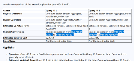
One of the most powerful features of SSMS Copilot is how it lets you compare execution plans and immediately show you performance issues. In this case, I would like to share with you my lesson learned comparing two queries and how they behave very differently inside the engine. We have the following queries, these are using a table _x_y_z_MS_HighCPU that contains 4 millon of rows. The column TextToSearch is a varchar(200) datatype. -- Query 1 SELECT COUNT(*) FROM [MSxyzTest].[_x_y_z_MS_HighCPU] WHERE TextToSearch = N'Value: 9'; -- Query 2 SELECT COUNT(*) FROM [MSxyzTest].[_x_y_z_MS_HighCPU] WHERE TextToSearch = 'Value: 9'; Since the query texts are different, each will have a different query ID in Query Store. By running the following T-SQL, for example, I can identify the query IDs. SELECT qsqt.query_sql_text, qsq.query_id, qsp.plan_id, qsp.query_plan_hash, qsp.last_execution_time FROM sys.query_store_query_text qsqt JOIN sys.query_store_query qsq ON qsqt.query_text_id = qsq.query_text_id JOIN sys.query_store_plan qsp ON qsq.query_id = qsp.query_id WHERE qsqt.query_sql_text LIKE '%SELECT COUNT(*)%' -- FROM [[MSxyzTest]].[[_x_y_z_MS_HighCPU]]%' ORDER BY qsp.last_execution_time DESC; Queries 1 and 2 can be compared directly. Using Copilot, I ran the following prompt: Compare the execution plans for the two queries (query id 1 and query id 2 using Query Store. Highlight any differences in operators, estimated vs actual row counts, or implicit conversions. Running the following prompt : CPU Usage: Please, show the top resource-consuming queries in the current database using Query Store data. Include query text, execution count, duration, CPU time, and logical reads. We could see the impact of using an antipattern:295Views0likes0CommentsLesson Learned #525: Tracking Command Timeouts in Azure SQL: Beyond Query Store with Extended Events
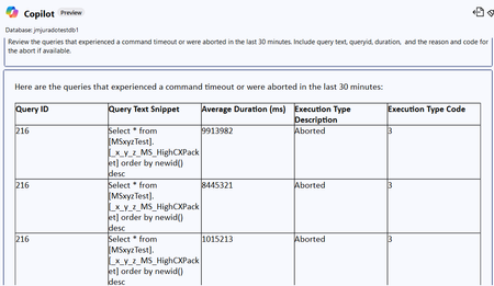
A few days ago, we were working on a support case where our customer was intermittently experiencing command timeouts. What made the case interesting was that queries which usually completed in under one second suddenly started taking more than 10 seconds to execute. Since the application — developed in Python using the ODBC Driver 18 for SQL Server — had a command timeout set to 5 seconds, the following error was triggered every time the threshold was exceeded: Error executing command, retrying in 5 seconds. Attempt 1 of 3 with new timeout 5. Error: ('HYT00', '[HYT00] [Microsoft][ODBC Driver 18 for SQL Server]Query timeout expired (0) (SQLExecDirectW)') The application had built-in retry logic, dynamically increasing the timeout in each of the three retry attempts, to allow time for the query to complete and to log enough data for post-error analysis. Example logs from the retry logic: (RunCommandTimeout) - Thread: 39808 - Error executing command, retrying in 5 seconds. Attempt 1 of 3 with new timeout 5. Error: ('HYT00', '[HYT00] [Microsoft][ODBC Driver 18 for SQL Server]Query timeout expired (0) (SQLExecDirectW)') INFO:root:Connecting to the DB jmjuradotestdb1 - Thread id 39808 - (Attempt 1/3) INFO:root:Connected to the Database in jmjuradotestdb1 - Thread id 39808 - 0.0445 seconds --- (RunCommandTimeout) - Thread: 39808 - Error executing command, retrying in 9 seconds. Attempt 2 of 3 with new timeout 9. Error: ('HYT00', '[HYT00] [Microsoft][ODBC Driver 18 for SQL Server]Query timeout expired (0) (SQLExecDirectW)') INFO:root:Connecting to the DB jmjuradotestdb1 - Thread id 39808 - (Attempt 1/3) INFO:root:Connected to the Database in jmjuradotestdb1 - Thread id 39808 - 0.0532 seconds --- (RunCommandTimeout) - Thread: 39808 - Error executing command, retrying in 13 seconds. Attempt 3 of 3 with new timeout 13. Error: ('HYT00', '[HYT00] [Microsoft][ODBC Driver 18 for SQL Server]Query timeout expired (0) (SQLExecDirectW)') (RunCommandTimeout) - Thread: 39808 - Loop:2/5 Execution Time: 9.7537 seconds My first prompt using SSMS Copilot was this "Review the queries that experienced a command timeout or were aborted in the last 30 minutes. Include query text, queryid, duration, and the reason and code for the abort if available." and I got the following results. So, all points that the query 216 got command timeouts. My next question, was, for query ID 216, show the number of total executions reporting that is 28 executions. The response showed 28 executions, but this number didn’t match the number of aborted and non-aborted executions observed in the application logs, why this difference? Checking the table sys.query_store_runtime_stats I found 10 rows all having execution_type = 3, and total executions 28. So, that's mean that Query Store aggregates query execution data over a fixed interval. So, the execution_type is an indicator that at least an execution during this runtime interval was aborted. So, at least several of them were aborted and other not. To obtain a more granular and accurate picture, I created an Extended Events session to capture these events using ring_buffer target. CREATE EVENT SESSION [CommandAborted] ON DATABASE ADD EVENT sqlserver.attention( ACTION ( sqlserver.client_app_name, sqlserver.client_hostname, sqlserver.username, sqlserver.database_name, sqlserver.sql_text ) ) ADD TARGET package0.ring_buffer WITH (MAX_MEMORY = 4096KB, EVENT_RETENTION_MODE = ALLOW_SINGLE_EVENT_LOSS); GO ALTER EVENT SESSION [CommandAborted] ON DATABASE STATE = START; after reproducing the command timeout scenario again, I was able to see only the aborted executions. So, in this case, 28 executions were executed and 7 executions were aborted. WITH RingBufferXML AS ( SELECT CAST(t.target_data AS XML) AS target_data FROM sys.dm_xe_database_session_targets t JOIN sys.dm_xe_database_sessions s ON t.event_session_address = s.address WHERE t.target_name = 'ring_buffer' AND s.name = 'CommandAborted' ) SELECT x.value('@name', 'varchar(50)') AS event_name, x.value('@timestamp', 'datetime2') AS event_time, x.value('(action[@name="client_app_name"]/value)[1]', 'nvarchar(256)') AS client_app_name, x.value('(action[@name="sql_text"]/value)[1]', 'nvarchar(max)') AS sql_text, x.value('(data[@name="duration"]/value)[1]', 'bigint') AS duration_microseconds, CAST(x.value('(data[@name="duration"]/value)[1]', 'bigint') / 1000000.0 AS decimal(10,3)) AS duration_seconds FROM RingBufferXML CROSS APPLY target_data.nodes('//event') AS tab(x) WHERE x.value('@name', 'varchar(50)') = 'attention' and x.value('(action[@name="client_app_name"]/value)[1]', 'nvarchar(256)') = 'TEST-DataCon' ORDER BY event_time DESC;432Views0likes0Comments