performance
131 TopicsGeneric Best Practices for HikariCP with Azure Database for PostgreSQL
Author: Mohamed Baioumy Technology: Azure Database for PostgreSQL (Flexible Server & Single Server) Category: Connectivity | Performance | Application Design Introduction Connection pooling is a critical component of application performance when connecting to Azure Database for PostgreSQL. Creating a new PostgreSQL connection is an expensive operation that consumes CPU, memory, and networking resources. Reusing existing connections through a connection pool significantly reduces connection latency, improves throughput, and helps applications scale more efficiently. Many Java applications use HikariCP, one of the most popular high-performance JDBC connection pools. While HikariCP provides excellent performance out of the box, improperly configured connection pool settings can lead to issues such as: Connection pool exhaustion Stale or invalid connections Increased connection acquisition latency Excessive connection creation and destruction Database resource contention Application timeouts This article summarizes generic guidance and best practices for configuring HikariCP when working with Azure Database for PostgreSQL Flexible Server and Azure Database for PostgreSQL Single Server. Understanding Key HikariCP Parameters 1. Maximum Lifetime (maxLifetime) The maxLifetime property controls how long a connection can remain in the pool before HikariCP retires it and creates a new one. Why It Matters Connections can become stale over time due to: Network interruptions Infrastructure updates Connection state changes TCP idle behavior Recycling connections periodically helps prevent applications from using long-lived connections that may no longer be healthy. Recommended Practice Avoid configuring the value too low. When maxLifetime is set aggressively, HikariCP continuously destroys and recreates connections, resulting in: Additional authentication overhead Increased connection establishment latency Higher CPU utilization Reduced application throughput A reasonable starting point is: spring.datasource.hikari.maxLifetime=1800000 30 minutes (1,800,000 ms) is commonly used and aligns well with many production workloads. Depending on workload characteristics, values between 30 minutes and 1 hour are generally suitable Avoid maxLifetime=300000 (5 minutes) This often causes unnecessary connection churn without providing additional benefits. 2. Minimum Idle Connections (minimumIdle) The minimumIdle setting defines how many idle connections HikariCP should keep ready for immediate use. Why It Matters A pool with available idle connections can serve application requests immediately without waiting for new connections to be established. However, maintaining too many idle connections consumes unnecessary database resources. Recommended Practice For most workloads: minimumIdle = maximumPoolSize Or minimumIdle slightly lower than maximumPoolSize This ensures sufficient connections are already available during traffic spikes while avoiding excessive connection creation delays. Example maximumPoolSize=20 minimumIdle=15 Avoid maximumPoolSize=20 minimumIdle=20 only when the application experiences long periods of inactivity and conserving resources is more important than immediate responsiveness. 3. Idle Timeout (idleTimeout) The idleTimeout property determines how long an unused connection remains in the pool before being removed. Why It Matters Connections that sit idle for extended periods consume resources on both: The application server Azure Database for PostgreSQL However, removing idle connections too quickly causes the application to repeatedly establish new connections. Recommended Practice Keep the default value unless there is a specific requirement. spring.datasource.hikari.idleTimeout=600000 which equals: 10 minutes (600,000 ms) This setting provides a good balance between resource utilization and responsiveness. [Re: EXT: R...0040002947 | Outlook] The timeout should also be comfortably longer than any expected short application idle periods. Avoid idleTimeout=10000 (10 seconds) Such aggressive settings often result in unnecessary connection creation cycles. 4. Maximum Pool Size (maximumPoolSize) This parameter determines the maximum number of concurrent database connections the application can maintain. Why It Matters This is often the most important HikariCP setting. If the Pool Is Too Small Applications may experience: Connection is not available, request timed out because all available connections are already in use. Similar scenarios have been observed during customer investigations involving Hikari pool exhaustion. If the Pool Is Too Large Applications can overwhelm the database server with excessive concurrent sessions, resulting in: Connection contention Increased context switching Higher memory consumption Reduced overall performance Recommended Practice Pool size should be based on: Database compute configuration CPU core count Query execution duration Application concurrency requirements Workload characteristics There is no universal value that fits every workload. Start conservatively: maximumPoolSize=10 or maximumPoolSize=20 maximumPoolSize=20 and increase only after load testing demonstrates a need for additional concurrency. Fixed-Size Pool Recommendation For many production workloads, a fixed-size pool provides the simplest and most predictable behavior. Configure: maximumPoolSize=20 minimumIdle=20 or omit minimumIdle entirely so it defaults to maximumPoolSize. HikariCP commonly recommends maintaining a fixed-size pool for responsiveness during demand spikes. Benefits Faster connection acquisition Predictable performance Reduced connection creation latency Better handling of traffic spikes When using a small fixed-size pool, there is often little need to aggressively tune: minimumIdle idleTimeout Instead, simply recycle connections using: maxLifetime maxLifetime Additional Recommendations Enable TCP Keepalive One common cause of stale connections is network devices silently dropping inactive TCP sessions. For PostgreSQL applications, consider enabling TCP keepalive: tcpKeepAlive=true tcpKeepAlive=true The HikariCP project specifically recommends enabling TCP keepalive to prevent rare situations where pools can lose valid connections. Monitor Connection Usage Track: Active connections Idle connections Connection acquisition time Pool exhaustion events Database connection counts These metrics help identify whether pool sizing is appropriate. Investigate Long-Running Queries Connection pool problems are often symptoms rather than root causes. A frequent scenario is: A query becomes slow. Connections remain occupied longer. The pool becomes exhausted. Applications start timing out. When analyzing HikariCP issues, always review: Query performance Blocking situations Database resource utilization Application connection handling logic Sample Production Configuration spring.datasource.hikari.maximumPoolSize=20 spring.datasource.hikari.minimumIdle=15 spring.datasource.hikari.maxLifetime=1800000 spring.datasource.hikari.idleTimeout=600000 spring.datasource.hikari.connectionTimeout=30000 spring.datasource.hikari.keepaliveTime=60000 spring.datasource.hikari.maximumPoolSize=20 spring.datasource.hikari.minimumIdle=15 spring.datasource.hikari.maxLifetime=1800000 spring.datasource.hikari.idleTimeout=600000 spring.datasource.hikari.connectionTimeout=30000 spring.datasource.hikari.keepaliveTime=60000 This configuration provides a solid starting point for many Azure Database for PostgreSQL workloads and can be adjusted based on application-specific requirements. a { text-decoration: none; color: #464feb; } tr th, tr td { border: 1px solid #e6e6e6; } tr th { background-color: #f5f5f5; } Conclusion HikariCP is extremely efficient when configured appropriately. The goal is not to maximize the number of connections, but rather to maintain a healthy balance between application responsiveness and database resource consumption. As a general rule: Use a reasonable maxLifetime (30–60 minutes) Keep enough idle connections available for traffic spikes Avoid aggressive idleTimeout values Size the pool based on workload characteristics, not guesses Consider fixed-size pools for predictable performance Monitor connection usage and query performance regularly By following these practices, applications connecting to Azure Database for PostgreSQL can achieve improved scalability, lower latency, and more reliable connectivity. References Connection pooling best practices - Azure Database for PostgreSQL Performance best practices for using Azure Database for PostgreSQL – Connection Pooling HikariCP Documentation and Pool Sizing GuidanceLessons Learned #540:Bulk Insert Throughput in Azure SQL Hyperscale with Partitioned Heap Tables
In this lesson learned, I would like to share an interesting scenario working on a service request where our customer was running a high-volume data load process in Azure SQL Database Hyperscale. The workload was based on a common pattern: Recreate a staging table. Load a large number of rows using bulk insert. The bulk insert showed unstable execution times and became the main area to investigate. The process was loading a very large number of rows into an Azure SQL Database Hyperscale database. The process used a staging table that was initially loaded as a heap. The main concern was the inconsistent execution time during the load process. Why Manually Adding Data Files Was Not the Right Direction In Azure SQL Database Hyperscale, the storage architecture is different from a traditional SQL Server deployment. The data layout and storage management are handled internally by the service. Because of this architecture, manually creating or pre-allocating multiple data files is not the same tuning option that we may consider in SQL Server on-premises or SQL Server running on Azure Virtual Machines. For this reason, the troubleshooting focus moved from manual file layout configuration to the actual workload pattern, waits, concurrency, batch size, and staging table design. What We Observed During the bulk insert phase, waits such as PAGELATCH_EX were observed. Since the staging table was loaded as a heap and the clustered primary key was created only after the bulk insert completed, OPTIMIZE_FOR_SEQUENTIAL_KEY was not directly applicable to the bulk insert phase. This changed the direction of the investigation. Instead of focusing on last-page insert contention on an existing clustered index, the analysis moved toward heap insert behavior, allocation contention, concurrency, batch size, and whether a different staging table design could help. First Recommendation: Start with Low-Impact Changes Before changing the table design, the first recommendation was to test the least intrusive changes: Reduce the number of concurrent bulk insert sessions. Increase the batch size, for example from 10,000 rows to 50,000 or 100,000 rows. Test TABLOCK on the dedicated heap staging table. The goal was to avoid assuming that more concurrency would always reduce the total execution time. In some high-volume load scenarios, excessive concurrency may increase contention and make the process less stable. The Interesting Design Option: Partitioned Heap Staging Table One of the most interesting design options was to evaluate a partitioned heap staging table. The idea is simple: instead of loading all rows into a non-partitioned heap staging table, the staging table can be created on the same partition scheme used by the target table, using the same partitioning column. This does not mean that a partitioned heap will always be faster. However, it can be a useful design option when: The bulk load phase is affected by allocation or latch contention. Concurrent load processes can naturally distribute rows across different partition ranges. The staging table is used only as an intermediate structure.Lessons Learned The main lessons from this scenario were: In Azure SQL Database Hyperscale, manually managing multiple data files is not the right tuning direction. PAGELATCH_EX during heap loading may point to concurrency or allocation-related contention. Reducing concurrency can sometimes improve total throughput. Larger batch sizes may provide better results than many small batches. TABLOCK on a dedicated heap staging table is a low-impact test worth evaluating. A partitioned heap staging table can be a valid second-phase design option when the load can be distributed across partition ranges. The best approach is to test small, measurable changes before introducing architectural redesigns. Final Thoughts A partitioned heap staging table can be a powerful option, but only when it is tested carefully and when the workload pattern can benefit from partition distribution.235Views0likes0CommentsLog Insights in Minutes: A Simpler pgBadger Workflow
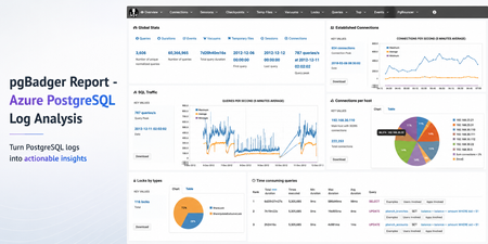
Sometimes the fastest way to understand a PostgreSQL workload is not another dashboard. It is a good log report. pgBadger is a PostgreSQL log analysis tool that turns raw PostgreSQL logs into an interactive HTML report. It helps summarize query activity, connection patterns, errors, temporary files, lock waits, autovacuum activity, and more. Earlier guidance for generating pgBadger reports from Azure Database for PostgreSQL Flexible Server focused on exporting logs through Diagnostic Settings, storing them in a storage account, and then using tools such as BlobFuse and jq to extract PostgreSQL log lines from JSON files. That workflow is still useful when customers centralize logs across multiple servers. However, if you are already using the Server logs feature in Azure Database for PostgreSQL Flexible Server, there is a much simpler path. In this post: You’ll learn how to generate a pgBadger HTML report from Azure Database for PostgreSQL Flexible Server by downloading native PostgreSQL .log files directly from the Azure portal. No storage account, BlobFuse mount, or JSON extraction required. Fast path Configure log_line_prefix . Enable Server logs for download. Download the PostgreSQL .log files. Run pgBadger with the matching prefix. Open pgbadger-report.html . Why use this workflow? With Server logs, you can download native PostgreSQL .log files directly from the Azure portal and run pgBadger locally. Older path Simpler path in this blog Diagnostic Settings → Storage account → BlobFuse → JSON extraction → pgBadger Server logs → Download .log files → pgBadger Area Older Diagnostic Settings workflow Server logs workflow Export path Diagnostic Settings to storage account Download .log files directly from the portal Format JSON payloads need extraction Native PostgreSQL .log files Extra tooling BlobFuse and jq JSON parsing None Best suited for Centralized or multi-server logging Quick per-server analysis Outcome Flexible, but more setup Faster path to pgBadger Recommended: Use the Server logs workflow when you want a fast, low-friction way to generate a pgBadger report from one Azure Database for PostgreSQL Flexible Server. When should you use this workflow? Use this workflow when... Use Diagnostic Settings when... You need a quick report for one Flexible Server. You centralize logs from many servers. You want to run pgBadger locally. You need long-term retention or workspace-level querying. You want to avoid JSON extraction. You already have automated log export pipelines. Before you start A machine where you can install or run pgBadger. A working Perl runtime. Git Bash on Windows, so the multi-line shell commands work as shown. Portal access to your Azure Database for PostgreSQL Flexible Server. Permission to update server parameters and enable Server logs. Important: pgBadger can only analyze what PostgreSQL logs capture. To populate query timing and slow-query sections in the report, enable log_min_duration_statement before collecting logs. Logs collected before that change will not include duration data. Workflow overview Task Type Rough effort Install or prepare pgBadger One-time setup per analysis machine 5–10 minutes Configure log_line_prefix One-time setup per server 2–3 minutes Enable Server logs One-time setup per server 2–3 minutes Download logs and run pgBadger Repeatable 2–5 minutes Install or prepare pgBadger on the machine where you will analyze logs. Configure log_line_prefix so pgBadger can parse each log line. Enable Server logs, so PostgreSQL logs are available for download. Download the logs and run pgBadger locally. 💡Pro tip: Start with a narrow log window first. Use one or two hourly log files, confirm the report looks right, and then expand the analysis window if needed. Step 1: Install pgBadger Before generating a report, you need pgBadger available on the machine where you plan to analyze the downloaded PostgreSQL log files. Run this on a Linux VM, WSL, or another Linux-based environment where you can install packages. Note: Azure Cloud Shell may work for quick testing, but package installation and build-tool availability can vary by session. For repeatable analysis, use a Linux VM, WSL, or another environment you control. Copy and run sudo apt-get update && sudo apt-get install -y git perl make gcc && \ git clone https://github.com/darold/pgbadger.git && \ cd pgbadger && \ perl Makefile.PL && \ make && \ sudo make install && \ pgbadger -V What good looks like: The install command completes successfully and pgbadger -V returns the installed pgBadger version. Step 2: Configure log_line_prefix This is a one-time server configuration step. The log_line_prefix parameter controls the beginning of each PostgreSQL log line. pgBadger uses this prefix to extract useful fields such as timestamp, user, database, and process ID. In the Azure portal, open your Flexible Server and go to Server parameters. Search for: Parameter log_line_prefix Set this value %m user=%u db=%d pid=%p: Then select Save. In Server parameters, confirm that the custom value is saved for log_line_prefix . Figure 1: Set log_line_prefix so pgBadger can correctly parse timestamp, user, database, and process ID from each log line. Prefix tokens Token Meaning %m Timestamp with milliseconds %u Username %d Database name %p Process ID After this change, log lines should look like this: Example log line 2026-06-22 19:00:00.070 UTC user=pgadmin db=highcpu pid=3805603: LOG: statement: SELECT 1 FROM pg_extension WHERE extname='pg_stat_statements' The matching pgBadger prefix for this log format is: Matching pgBadger prefix %m user=%u db=%d pid=%p: You will use this same value later in the pgBadger command. What good looks like: The server parameter is saved, and new PostgreSQL log lines begin with timestamp, user, database, and process ID fields that match the pgBadger prefix. Step 3: Enable Server logs for download This is also a one-time setup step. In the Azure portal, open your Flexible Server and go to Server logs. Enable: Portal setting Capture logs for download Set the retention period based on how long you want logs to remain available for download. For example, a 7-day retention period keeps logs available for download for 7 days. In Server logs, enable Capture logs for download and choose the retention window. Figure 2: Enable Capture logs for download and set a retention period long enough to cover the analysis window you want to inspect. What good looks like: After Server logs are enabled, hourly PostgreSQL log files appear in the Server logs blade and can be downloaded from the Azure portal. Once enabled, hourly log files appear in the Server logs blade. The files are named by date and hour, for example: Example log files postgresql_2026_06_22_19_00_00.log postgresql_2026_06_22_20_00_00.log Step 4: Download and organize the logs locally From the Server logs page, select the .log files for the time window you want to analyze and download them. For example, to analyze activity between 19:00 and 21:00 UTC, download: Example files to download postgresql_2026_06_22_19_00_00.log postgresql_2026_06_22_20_00_00.log On your local machine, create a folder for that analysis window. A simple convention is to use the Mon-DD format. Folder name Jun-22 Place the downloaded .log files inside that folder. Your local folder structure should look like this: Folder structure pgbadger-13.1/ pgbadger Jun-22/ postgresql_2026_06_22_19_00_00.log postgresql_2026_06_22_20_00_00.log Step 5: Generate the pgBadger report Open Git Bash from the folder where pgBadger is located. For example, if pgBadger is inside the pgbadger-13.1 folder, open Git Bash from that folder. # Action Command 1 Set the folder FOLDER=Jun-22 2 Confirm files ls -lh ./$FOLDER 3 Run pgBadger Use the full command below. Copy and run FOLDER=Jun-22 ls -lh ./$FOLDER perl -X ./pgbadger -f stderr \ --prefix '%m user=%u db=%d pid=%p:' \ ./$FOLDER/*.log \ -o ./$FOLDER/pgbadger-report.html Command breakdown Part of command Purpose perl -X ./pgbadger Runs pgBadger and suppresses non-critical Perl warnings. -f stderr Parses PostgreSQL stderr log files. --prefix '%m user=%u db=%d pid=%p:' Matches the log_line_prefix set on the server. ./$FOLDER/*.log Analyzes every .log file in the selected folder. -o ./$FOLDER/pgbadger-report.html Writes the HTML report into the same folder. When the command completes successfully, you should see output like this: Expected output Parsed 12134249 bytes of 12134249 (100.00%), queries: 26684, events: 83 LOG: Ok, generating html report... What good looks like: pgBadger finishes parsing the logs and creates pgbadger-report.html in the selected folder. Step 6: Open the report Open the generated report: Copy and run start ./$FOLDER/pgbadger-report.html The report opens in your default browser. The final report is created here: Generated report path Jun-22/pgbadger-report.html What the report can show The pgBadger report gives you a quick view into the workload shape for the selected log window. For example, in a sample run across two hourly log files, pgBadger summarized: Total number of queries. Number of unique normalized queries. Query traffic over time. Events such as errors and fatal messages. Session and connection patterns. Once the report opens, start with Global Stats to confirm the time range, total queries, normalized queries, and query peak. Figure 3: Start with Global Stats to validate the selected time range, total query count, normalized query count, and query peak. Query volume and normalized queries Many raw queries can often reduce to a smaller number of normalized query patterns. This helps identify whether the workload is spread across many different query shapes or dominated by a smaller set of repeated statements. Example: In this sample run, 26,684 queries reduced to 59 normalized query shapes. That suggests the workload is mostly a small set of repeated statements, which can help focus tuning effort. Traffic patterns The SQL Traffic section helps identify spikes, quiet periods, and workload changes over time. Figure 4: Use SQL Traffic to identify query spikes, quiet periods, and workload changes during the selected log window. Figure 5: Review the query breakdown to compare read vs. write volume and query-type distribution for the selected Server logs window. For example, if the report shows a steady baseline followed by a sharp spike, that spike can be correlated with application activity, batch jobs, synthetic tests, or operational events during the same time window. Query duration If query duration shows 0 ms or the slow query sections are empty, it usually means duration logging was not enabled when the logs were collected. In that case, pgBadger can still show query counts and events, but it cannot calculate the slowest queries, total execution time, average duration, or maximum duration. To unlock those timing sections, enable log_min_duration_statement , collect fresh logs, and rerun pgBadger. What pgBadger cannot infer from missing logs pgBadger reports are only as complete as the log data you provide. If PostgreSQL did not log duration, lock waits, temporary files, or autovacuum activity during the selected time window, pgBadger cannot reconstruct those details later. To analyze... Enable before collecting logs Slow queries log_min_duration_statement Lock waits log_lock_waits Temporary files log_temp_files Autovacuum activity log_autovacuum_min_duration Repeatable copy/paste block Reusable command block Change only FOLDER for each new analysis window. Copy and run FOLDER=Jun-22 ls -lh ./$FOLDER perl -X ./pgbadger -f stderr \ --prefix '%m user=%u db=%d pid=%p:' \ ./$FOLDER/*.log \ -o ./$FOLDER/pgbadger-report.html start ./$FOLDER/pgbadger-report.html For another date, change only this line: Update this value FOLDER=Jun-22 Examples: Example folder values FOLDER=Jun-23 FOLDER=Jul-01 FOLDER=Aug-15 Optional: Improve report quality pgBadger can only analyze the information captured in PostgreSQL logs. The default logs may be enough for query frequency, connection activity, and errors. For deeper performance troubleshooting, consider enabling additional logging parameters based on your scenario. Scenario Parameter Suggested value Notes Slow query analysis log_min_duration_statement 1000 Logs statements slower than 1 second. Short controlled test log_min_duration_statement 0 Logs every statement. Use carefully. Lock troubleshooting log_lock_waits on Helps identify lock waits. Temporary file analysis log_temp_files 0 Logs all temporary files. Autovacuum visibility log_autovacuum_min_duration 0 Useful during focused analysis. Useful parameters include: Recommended logging parameters log_lock_waits = on log_temp_files = 0 log_autovacuum_min_duration = 0 To capture query durations, configure: Duration logging log_min_duration_statement = 1000 This logs statements that run longer than 1000 milliseconds. For short test runs, you can temporarily use: Short test run only log_min_duration_statement = 0 Caution: Use log_min_duration_statement = 0 carefully on busy production servers. It logs every statement and can generate a large volume of logs. Duration matters: If duration logging is not enabled, pgBadger can still show query counts and events, but slowest-query, total duration, average duration, and maximum duration sections will be limited or empty. Common mistakes and quick fixes Symptom Likely cause Fix Report is empty Prefix mismatch Match --prefix with log_line_prefix . No duration data Duration logging was not enabled Set log_min_duration_statement before collecting logs. No files visible Server logs disabled or retention expired Enable capture and check retention. pgBadger command fails pgBadger is not in the current folder or path Run pgbadger -V to confirm installation. Common troubleshooting FAQs 1. Report is created but empty This usually means the pgBadger prefix did not match the actual log format. Check the first few lines: Copy and run head -5 ./$FOLDER/*.log Make sure the pgBadger --prefix matches the server’s log_line_prefix . 2. Report shows queries but no duration PostgreSQL logged statements but did not log durations. Enable one of the following, collect fresh logs, and rerun pgBadger: Parameter options log_min_duration_statement = 1000 # or temporarily for testing log_min_duration_statement = 0 3. No .log files are visible Confirm that Server logs are enabled: Portal setting Capture logs for download Also check the retention period. If the retention period has expired, older logs may no longer be available for download. 4. pgBadger command fails Confirm that pgBadger is available in the current folder or installed in your path. Copy and run pgbadger -V If you are running pgBadger from the local folder, use: Copy and run perl -X ./pgbadger Summary For customers already using Azure Database for PostgreSQL Flexible Server logs, the pgBadger workflow is straightforward: Install pgBadger. Configure log_line_prefix . Enable Server logs for download. Download the .log files. Place them in a local date-based folder. Run pgBadger with the matching prefix. Open pgbadger-report.html . Bottom line: Server logs give you the shortest path from Azure Database for PostgreSQL Flexible Server logs to a pgBadger report. Download the native .log files, run pgBadger with the matching prefix, and open the generated HTML report. References pgBadger - source and documentation GitHub pgBadger - project site Azure - Download server logs from the portal Flexible Server Azure - Logging concepts Flexible Server Azure - Configure server parameters via the portal PostgreSQL - log_line_prefix and logging parameters674Views2likes0CommentsLessons Learned #547:Some SQL DB Statistics Remain Outdated While Others Are Automatically Updated
During the analysis of a SQL Server performance case, we observed an interesting statistics update pattern on a large table. Several statistics had recently been updated at different times, while a group of automatically created _WA_Sys_ statistics still showed: An older last_updated date. A high modification_counter. A row count significantly lower than the current number of rows in the table. At first glance, this could suggest that AUTO_UPDATE_STATISTICS was not working correctly. However, a closer review showed that this pattern can be completely consistent with the expected behavior of SQL Server. 1. Types of statistics in SQL Server SQL Server can maintain several types of statistics. Automatically created column statistics When AUTO_CREATE_STATISTICS is enabled, SQL Server can automatically create a single-column statistic when the Query Optimizer needs cardinality information for a column used in a query predicate. These statistics normally use names such as: _WA_Sys_00000002_47A6D5E5 The name can be interpreted as: _WA_Sys_<column_id in hexadecimal>_<object_id in hexadecimal> For example: 00000002 hexadecimal = column_id 2 47A6D5E5 hexadecimal = table object_id The most reliable way to identify the associated column is not to decode the name manually, but to query the SQL Server catalog views: DECLARE @TableName sysname = N'dbo.CustomerTransactions'; SELECT s.stats_id, s.name AS statistics_name, sc.stats_column_id, c.column_id, c.name AS column_name, s.auto_created, s.user_created, s.no_recompute FROM sys.stats AS s INNER JOIN sys.stats_columns AS sc ON sc.object_id = s.object_id AND sc.stats_id = s.stats_id INNER JOIN sys.columns AS c ON c.object_id = sc.object_id AND c.column_id = sc.column_id WHERE s.object_id = OBJECT_ID(@TableName) AND s.name = N'_WA_Sys_00000002_47A6D5E5' ORDER BY sc.stats_column_id; Statistics associated with indexes When SQL Server creates an index, it also creates a statistics object associated with the index. For example: CREATE INDEX IX_CustomerTransactions_ClientId ON dbo.CustomerTransactions(ClientId) this creates an index statistics object normally named: IX_CustomerTransactions_ClientId when a statistics object corresponds to an index, its stats_id matches the index's index_id. User-created statistics Statistics can also be created explicitly: CREATE STATISTICS ST_CustomerTransactions_ClientId_Status ON dbo.CustomerTransactions ( ClientId, StatusId ); This object is identified in sys.stats with: user_created = 1 auto_created = 0 and AUTO_UPDATE_STATISTICS applies to index statistics, automatically created single-column statistics, manually created statistics and filtered statistics. 2. Statistics are not updated together Assume that a table has these statistics: _WA_Sys_00000002_xxxxxxxx for ClientId _WA_Sys_00000003_xxxxxxxx for StatusId IX_CustomerTransactions_CreatedDate for CreatedDate PK_CustomerTransactions and TransactionId After a large data load, several or all of them could become eligible for an automatic update. However, SQL Server does not immediately update all eligible statistics. Before compiling a query, the Query Optimizer identifies the statistics that could be relevant to the query predicates and checks whether those statistics are outdated. Consider this query: SELECT TransactionId, ClientId, Amount FROM dbo.CustomerTransactions WHERE ClientId = 100; The optimizer might need a histogram on ClientId. If the corresponding statistics object is outdated and has crossed its update threshold, SQL Server may update that specific statistics object. It does not need to update unrelated statistics on: StatusId CreatedDate As a result, statistics on the same table can legitimately have different update times: PK_CustomerTransactions 2026-07-22 10:53 IX_CustomerTransactions_ClientId 2026-07-22 10:50 IX_CustomerTransactions_CreatedDate 2026-07-22 10:13 _WA_Sys_00000003_47A6D5E5 2026-07-19 10:00 This pattern can be evidence of demand-driven automatic updates rather than evidence of a malfunction. 3. What does modification_counter represent? The modification_counter returned by sys.dm_db_stats_properties represents the number of modifications made to the leading statistics column since that statistics object was last updated. This definition is especially important for multicolumn statistics. For example: CREATE INDEX IX_CustomerTransactions_ClientId_Status ON dbo.CustomerTransactions ( ClientId, StatusId ); The associated statistics object contains: Histogram: ClientId Density information: ClientId ClientId, StatusId The histogram and modification_counter are based on the leading column, ClientId. If only StatusId is modified: UPDATE dbo.CustomerTransactions SET StatusId = 2 WHERE TransactionId = 100; this does not have the same statistics impact as changing ClientId, because ClientId is the leading histogram column. SQL Server statistics contain only one histogram, built on the first key column. Multicolumn statistics additionally contain density information for column prefixes. 4. Why do multiple statistics sometimes have similar modification counters? This commonly happens after an insert operation. For example: INSERT INTO dbo.CustomerTransactions ( TransactionId, ClientId, StatusId, Amount, CreatedDate ) SELECT TransactionId, ClientId, StatusId, Amount, CreatedDate FROM dbo.StagingCustomerTransactions; Each inserted row introduces a value for every populated column. Consequently, multiple single-column statistics may show similar increases in their modification counters. This is particularly visible after a large ETL operation: Table rows before the load: 487,673 Rows inserted by the ETL: 515,244 Current approximate row count: 1,002,917 Several statistics could then show modification counters close to the number of inserted rows. That does not mean SQL Server must update all those statistics immediately. They become candidates for updating, but an update is normally triggered when query optimization requires them. 5. Does automatic updating apply only to _WA_Sys_ statistics? AUTO_UPDATE_STATISTICS applies to: Automatically created _WA_Sys statistics Index statistics Primary-key index statistics User-created statistics Each statistics object is evaluated independently. Therefore, SQL Server might update: PK_CustomerTransactions while leaving this object unchanged: _WA_Sys_00000003_47A6D5E5 The reverse is also possible. The behavior depends on which statistics are considered relevant during compilation or cached-plan validation. 6. What happens when a _WA_Sys_ statistic and an index statistic cover the same column? This is one of the most interesting scenarios. Assume SQL Server originally created: _WA_Sys_00000002_xxxxxxxx for ClientId. Later, someone creates this index: CREATE INDEX IX_CustomerTransactions_ClientId ON dbo.CustomerTransactions(ClientId); The table now has two statistics objects with histograms on ClientId: _WA_Sys_00000002_xxxxxxxx and IX_CustomerTransactions_ClientId Conceptually: _WA_Sys statistic Histogram on ClientId Index statistic Histogram on ClientId For a query such as: SELECT * FROM dbo.CustomerTransactions WHERE ClientId = @ClientId; the optimizer can have more than one potentially relevant statistics object. It may rely on the index statistics object rather than the older _WA_Sys_ object. In that case: IX_CustomerTransactions_ClientId Updated recently _WA_Sys_00000002_xxxxxxxx Old last_updated value High modification_counter This does not necessarily mean that automatic statistics updating has failed. It can mean that the _WA_Sys_ statistic has become redundant and has not been required by recent compilations. However, this should be presented carefully: The Query Optimizer is not publicly documented as always preferring an index statistic over an equivalent _WA_Sys_ statistic. The statistics selected can depend on: Query. Predicates. Available indexes. Filtered versus unfiltered statistics. Statistics freshness. Sampling quality. Multicolumn density information. Cardinality Estimator behavior. Existing cached plans. The correct conclusion is that the scenario is possible and plausible, but the execution plan should be inspected before claiming that a specific statistics object was used. As we wrote down in multiple articles in our blog (below), identify redudant statistics is part of DBA work to avoid this situation, also, in other situations, I saw that the maintenance plan is taking too much time because we are updating statistics that we are not using or migth be duplicated. The following script identifies statistics whose leading columns overlap: DECLARE @TableName sysname = N'dbo.CustomerTransactions'; ;WITH LeadingStatisticsColumns AS ( SELECT s.object_id, s.stats_id, s.name AS statistics_name, s.auto_created, s.user_created, s.no_recompute, s.has_filter, s.filter_definition, sc.column_id, c.name AS leading_column, i.index_id, i.name AS index_name FROM sys.stats AS s INNER JOIN sys.stats_columns AS sc ON sc.object_id = s.object_id AND sc.stats_id = s.stats_id AND sc.stats_column_id = 1 INNER JOIN sys.columns AS c ON c.object_id = sc.object_id AND c.column_id = sc.column_id LEFT JOIN sys.indexes AS i ON i.object_id = s.object_id AND i.index_id = s.stats_id WHERE s.object_id = OBJECT_ID(@TableName) ) SELECT leading_column, statistics_name, CASE WHEN index_id IS NOT NULL THEN N'INDEX STATISTICS' WHEN auto_created = 1 THEN N'AUTO-CREATED _WA_SYS' WHEN user_created = 1 THEN N'USER-CREATED STATISTICS' ELSE N'OTHER' END AS statistics_type, index_name, has_filter, filter_definition, no_recompute, COUNT(*) OVER ( PARTITION BY column_id ) AS statistics_on_same_leading_column FROM LeadingStatisticsColumns ORDER BY leading_column, statistics_type, statistics_name; This does not automatically mean that one object should be deleted. It only identifies an overlap. 7. Script The following example demonstrates how an automatically created statistic can coexist with a later index statistic. DROP TABLE IF EXISTS dbo.CustomerTransactions; GO CREATE TABLE dbo.CustomerTransactions ( TransactionId int NOT NULL, ClientId int NOT NULL, StatusId tinyint NOT NULL, Amount decimal(12,2) NOT NULL, CreatedDate datetime2(0) NOT NULL, CONSTRAINT PK_CustomerTransactions PRIMARY KEY CLUSTERED (TransactionId) ); GO Insert sample data ;WITH Numbers AS ( SELECT TOP (200000) ROW_NUMBER() OVER ( ORDER BY (SELECT NULL) ) AS n FROM sys.all_objects AS a CROSS JOIN sys.all_objects AS b ) INSERT INTO dbo.CustomerTransactions ( TransactionId, ClientId, StatusId, Amount, CreatedDate ) SELECT n, n % 5000, n % 5, CONVERT(decimal(12,2), n % 10000), DATEADD ( minute, -(n % 100000), SYSUTCDATETIME() ) FROM Numbers; GO Ensure that automatic statistics creation and updating are enable ALTER DATABASE CURRENT SET AUTO_CREATE_STATISTICS ON; GO ALTER DATABASE CURRENT SET AUTO_UPDATE_STATISTICS ON; GO Trigger automatic statistics creation on ClientId SELECT COUNT_BIG(*) FROM dbo.CustomerTransactions WHERE ClientId = 100 OPTION (RECOMPILE); GO Check the statistics created for ClientId SELECT s.stats_id, s.name AS statistics_name, s.auto_created, s.user_created, c.name AS column_name FROM sys.stats AS s INNER JOIN sys.stats_columns AS sc ON sc.object_id = s.object_id AND sc.stats_id = s.stats_id INNER JOIN sys.columns AS c ON c.object_id = sc.object_id AND c.column_id = sc.column_id WHERE s.object_id = OBJECT_ID(N'dbo.CustomerTransactions') AND c.name = N'ClientId' ORDER BY s.stats_id; Create an index on the same column CREATE INDEX IX_CustomerTransactions_ClientId ON dbo.CustomerTransactions(ClientId); The table can now have: Modify the data significantly UPDATE dbo.CustomerTransactions SET ClientId = ClientId + 10000 WHERE TransactionId <= 100000; Review the counters again SELECT s.name AS statistics_name, sp.last_updated, sp.rows, sp.rows_sampled, sp.modification_counter FROM sys.stats AS s OUTER APPLY sys.dm_db_stats_properties ( s.object_id, s.stats_id ) AS sp WHERE s.object_id = OBJECT_ID(N'dbo.CustomerTransactions') ORDER BY s.stats_id Force a new compilation using ClientId SET STATISTICS XML ON; GO SELECT COUNT_BIG(*) FROM dbo.CustomerTransactions WHERE ClientId = 10100 OPTION (RECOMPILE); GO SET STATISTICS XML OFF; GO After the query, review: The actual execution plan XML. The StatisticsInfo elements. last_updated. modification_counter. The exact object updated is an optimizer decision and can vary by SQL Server version, build, compatibility level and query shape. The test should therefore be used to observe the behavior rather than to assume a fixed preference. Finally, as you could see SQL Server choose _WA_Sys_00000002_151102AD instead of IX_CustomerTransactions_ClientId to update. In some situations, depending on execution plan, SQL Server might choose IX_CustomerTransactions_ClientId to update instead of _WA_Sys_00000002_151102AD and for this reason, doesn't mean that SQL Server is not updating the statistics it is depending that it is choosing one of them that the column is involved. My lessons learned, a statistic can be outdated without being relevant, and it can be relevant without being the only available source of cardinality information. Before interpreting an old last_updated value as an automatic statistics failure, identify the leading column, look for overlapping statistics, inspect the execution plan and determine whether there is a real estimation or performance problem. Articles: Lesson Learned #482: Identifying Potential Duplicate Statistics | Microsoft Community Hub Lesson Learned #324: Query Recompilation in Azure SQL | Microsoft Community Hub Lessons Learned #537: Copilot Prompts for Troubleshooting on Azure SQL Database | Microsoft Community Hub Lesson Learned #498:Understanding the Role of STATMAN in SQL Server and Its Resource Consumption | Microsoft Community Hub Disclaimer: The scripts included in this article are provided for demonstration and educational purposes only. They create a sample table, insert a significant number of rows, create indexes and statistics, modify data, and change automatic statistics settings in the current database. Run the complete demonstration only in a test or non-production environment. Review and adapt the database name, object names, row volume, and statements before execution. The results may vary depending on the SQL Server version, database compatibility level, existing configuration, data distribution, and workload. Always test the scripts in a representative environment before applying any conclusion or change to a production system.303Views0likes0CommentsLessons Learned #544: How to Detect INT Identity Exhaustion Before Inserts Fail.
Recently, I worked on a support case involving an Azure SQL Database table where the customer had reached the maximum value supported by the INT data type. The table used an INT IDENTITY(1,1) column as its primary key. Over time, the generated identity value approached the maximum value supported by INT. Once the available range was exhausted, the application was no longer able to insert new rows. At that point, the column needed to be changed from INT to BIGINT. However, performing this type of migration on a very large table can be a complex and time-consuming operation. The situation is that an INT column uses 4 bytes and supports values from: -2,147,483,648 to: 2,147,483,647. To prevent similar problems in the future, I suggested using the following query to review the current status of all INT IDENTITY columns in the database. The query uses the sys.identity_columns catalog view: SELECT s.name AS SchemaName, t.name AS TableName, c.name AS ColumnName, CONVERT(bigint, c.last_value) AS CurrentIdentityValue, CONVERT(bigint, 2147483647) AS MaximumIntValue, CONVERT(bigint, 2147483647) - ISNULL(CONVERT(bigint, c.last_value), 0) AS RemainingValues, CAST( ISNULL(CONVERT(decimal(20,2), c.last_value), 0) / 2147483647 * 100 AS decimal(6,2) ) AS PercentUsed FROM sys.identity_columns AS c INNER JOIN sys.tables AS t ON c.object_id = t.object_id INNER JOIN sys.schemas AS s ON t.schema_id = s.schema_id WHERE TYPE_NAME(c.system_type_id) = 'int' ORDER BY PercentUsed DESC; I prefer using this query instead of relying on: SELECT COUNT(*) FROM dbo.TableName. The number of rows in a table does not necessarily match the current identity value. Rows might have been deleted, transactions might have been rolled back, and identity values might contain gaps. For this reason, the current identity value is a better indicator of the remaining capacity. Adding this query as a regular preventive check can help identify identity columns that are approaching their limits before they cause application failures. I would like to share with you an example creates a table with an identity seed close to the maximum value supported by INT: DROP TABLE IF EXISTS dbo.IdentityCapacityDemo2; CREATE TABLE dbo.IdentityCapacityDemo2 ( Id INT IDENTITY(2147483600,1) NOT NULL, CreatedDate datetime2(0) NOT NULL CONSTRAINT DF_IdentityCapacityDemo2_CreatedDate DEFAULT SYSUTCDATETIME(), CONSTRAINT PK_IdentityCapacityDemo2 PRIMARY KEY CLUSTERED (Id) ) Insert 20 rows using this command: insert into IdentityCapacityDemo2(CreatedDate) values(SYSUTCDATETIME()) Example of returns: I think runnning this preventive check can help detect identity exhaustion before it affects the application.Lessons Learned #541:Automatic Plan Correction vs External Tables: A Practical Lesson from the Field
Automatic Plan Correction is one of the most useful capabilities in Azure SQL Database when dealing with plan regressions. It uses Query Store to identify when a query starts using a worse execution plan and, when appropriate, forces the last known good plan. However, during a recent troubleshooting scenario, I found that not all queries have the same execution characteristics. In particular, queries that reference external tables may behave differently from fully local queries because part of their execution depends on remote data access. When Query Store is configured to capture all queries, we can use it to identify queries that reference external tables and review whether those query IDs should participate in FORCE_LAST_GOOD_PLAN. From a practical perspective, external-table queries may not always be the best candidates for Automatic Plan Correction, especially when the expected benefit of automatic plan forcing is not clear. For that reason, the goal of this article is simple: identify queries that reference external tables and, when appropriate, exclude selected query IDs from Automatic Plan Correction. If we review the execution plan for the following query: DECLARE @Region nvarchar(50) = N'EMEA' SELECT CustomerId, CustomerName, Region FROM dbo.ExternalCustomers WHERE Region = @Region; We can see that the plan includes a Remote Query operator. This means that the query is not only accessing local data; part of the execution depends on remote data access through the external table. For this type of query, Automatic Plan Correction may not provide the same clear benefit as it does for fully local queries. The performance may depend not only on the local execution plan, but also on the remote database, the external data source, network latency, and the amount of data returned from the remote side. For that reason, queries referencing external tables are good candidates for review before allowing them to participate in FORCE_LAST_GOOD_PLAN. In this scenario, the first step was to identify the Query Store query_id associated with the query referencing the external table. Since the query text was available in Query Store, we searched for the external table name in sys.query_store_query_text. SELECT q.query_id, p.plan_id, p.is_forced_plan, p.plan_forcing_type_desc, p.force_failure_count, p.last_force_failure_reason_desc, p.last_execution_time, qt.query_sql_text FROM sys.query_store_query_text AS qt INNER JOIN sys.query_store_query AS q ON qt.query_text_id = q.query_text_id INNER JOIN sys.query_store_plan AS p ON q.query_id = p.query_id WHERE qt.query_sql_text LIKE N'%ExternalCustomers%' ORDER BY p.last_execution_time DESC; Once the query_id was identified, the next step was to exclude that specific query from Automatic Plan Correction by setting FORCE_LAST_GOOD_PLAN to OFF for that query_id. EXECUTE sys.sp_configure_automatic_tuning @option = 'FORCE_LAST_GOOD_PLAN', @type = 'QUERY', @type_value = N'<query_id>', @option_value = 'OFF'; For example: EXECUTE sys.sp_configure_automatic_tuning @option = 'FORCE_LAST_GOOD_PLAN', @type = 'QUERY', @type_value = N'1574', @option_value = 'OFF'; This does not disable Automatic Plan Correction for the entire database. It only tells Automatic Plan Correction to ignore this specific Query Store query ID for FORCE_LAST_GOOD_PLAN. With this approach, Automatic Plan Correction can remain enabled for the rest of the database workload, while selected queries that depend on external or remote data access can be reviewed and excluded individually when automatic plan forcing is not expected to provide a clear benefit.161Views0likes0CommentsScaling Write Throughput in Azure Database for MySQL Using Application-Level Sharding
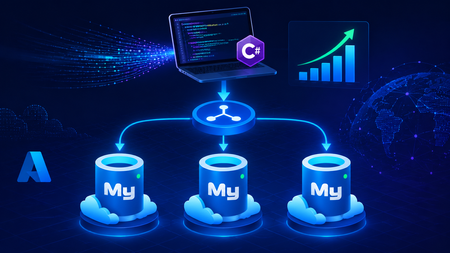
This blog post walks through scaling write throughput in Azure Database for MySQL using application level sharding. It starts with the why behind sharding and then builds a complete C# implementation that spreads writes across three Azure Database for MySQL Flexible Servers. Why Shard in the First Place? This post focuses specifically on scaling write throughput. A well-tuned single primary node can take you remarkably far, and techniques such as indexing strategies, write batching, redo log optimization, and vertical compute scaling each deliver real, lasting value. For many workloads, these optimizations are all you will ever need. That said, as write volume continues to grow, a single primary eventually approaches its practical capacity, and at that point the most durable way to keep scaling is to distribute the write workload across multiple primary instances. This architecture is what we call sharding. When you reach this inflection point, there are two primary patterns for managing multiple write nodes: Proxy or Middleware Layer Sharding: A sharding aware proxy sits between the application and a pool of Azure Database for MySQL instances, routing queries based on a shard key. While this abstracts the underlying topology from the application layer, it introduces an additional, complex component to operate, secure, scale, and patch. Application Layer Sharding: The application itself resolves the destination shard key and determines which of the N Azure Database for MySQL instances should receive a write before ever opening a database connection. Each backend target remains a completely standard, independent Azure Database for MySQL instance. This post explores the second approach. The core appeal of application layer sharding is architectural simplicity: it introduces zero infrastructure overhead and eliminates an extra network hop. Every shard behaves exactly like a standalone instance, meaning your existing backup, restore, monitoring pipelines, and the Azure portal function seamlessly without modification. The explicit tradeoff is that you forgo cross shard joins and distributed transactions in exchange for absolute predictability and control over data access patterns. The Plan We will build a small order management service that distributes its data across three Azure Database for MySQL instances that already exist. The application, written in C# on .NET 8, owns the partitioning logic. The premise: the three servers are already provisioned, the firewalls are configured, the network paths are established, and each server has its own administrative credentials. We are not provisioning infrastructure in this post. we are writing the application code that consumes it. mysql-shard-0.mysql.database.azure.com user: shard0_admin pwd: <secret-0> mysql-shard-1.mysql.database.azure.com user: shard1_admin pwd: <secret-1> mysql-shard-2.mysql.database.azure.com user: shard2_admin pwd: <secret-2> Each server hosts an identical appdb database with the same schema: CREATE TABLE users ( user_id BIGINT NOT NULL PRIMARY KEY, email VARCHAR(255) NOT NULL, created_at DATETIME NOT NULL DEFAULT CURRENT_TIMESTAMP, UNIQUE KEY uq_email (email) ); CREATE TABLE orders ( order_id BIGINT NOT NULL PRIMARY KEY, user_id BIGINT NOT NULL, amount_cents INT NOT NULL, created_at DATETIME NOT NULL DEFAULT CURRENT_TIMESTAMP, KEY ix_user (user_id) ); Two design decisions in this schema warrant explanation: No AUTO_INCREMENT for user_id or order_id. Two shards would otherwise generate the same value 42 independently. Instead, we assign identifiers in the application, using a scheme such as Snowflake, ULID, or UUIDv7. orders carries user_id, and we route by it. This is the single most important rule of sharding: choose a shard key that keeps related data colocated, so that the common queries remain on a single shard. A note on UNIQUE KEY uq_email. A unique index enforces uniqueness only within a single physical shard. Because we route by user_id, two users with different IDs and the same email may land on different shards, and both inserts will succeed. If you require globally unique emails, two options exist: (a) maintain a separate email → user_id lookup table on a single "directory" server and write to it first within an idempotent flow, or (b) shard the users table by a hash of email instead. We retain user_id routing throughout this post because it is the correct choice for orders, and we treat per shard email uniqueness as a best effort guard rather than a hard global invariant. How the Partitioning Works The naive approach to sharding is shard = hash(key) % N. This works until you need to add a fourth server, at which point roughly 75% of your data must move. In any system of meaningful size, that is prohibitively expensive. The established solution is virtual buckets. You hash the key into a large, fixed bucket space (here, 1024), then map buckets to physical shards. When you add capacity, you relocate only buckets; you never rehash the entire dataset. In production, the bucket_to_shard_map typically resides in a system such as Azure App Configuration or etcd, so that you can rebalance without redeploying. For this post, we keep it as an in-memory array seeded at startup, which is straightforward to replace later. The Project ShardingDemo/ ├── ShardingDemo.csproj ├── appsettings.json ├── Models.cs ├── ShardRouter.cs ├── UserRepository.cs └── Program.cs ShardingDemo.csproj <Project Sdk="Microsoft.NET.Sdk"> <PropertyGroup> <OutputType>Exe</OutputType> <TargetFramework>net8.0</TargetFramework> <Nullable>enable</Nullable> <ImplicitUsings>enable</ImplicitUsings> </PropertyGroup> <ItemGroup> <PackageReference Include="MySqlConnector" Version="2.6.0" /> <PackageReference Include="Microsoft.Extensions.Hosting" Version="8.0.0" /> <PackageReference Include="Microsoft.Extensions.Configuration.Binder" Version="8.0.0" /> </ItemGroup> <ItemGroup> <Content Include="appsettings.json" CopyToOutputDirectory="PreserveNewest" /> </ItemGroup> </Project> appsettings.json Shards is an ordered list, and a shard's position in the array is its logical ID. { "Shards": [ { "Host": "mysql-shard-0.mysql.database.azure.com", "Database": "appdb", "User": "shard0_admin", "Password": "REPLACE_ME_0" }, { "Host": "mysql-shard-1.mysql.database.azure.com", "Database": "appdb", "User": "shard1_admin", "Password": "REPLACE_ME_1" }, { "Host": "mysql-shard-2.mysql.database.azure.com", "Database": "appdb", "User": "shard2_admin", "Password": "REPLACE_ME_2" } ] } Models.cs namespace ShardingDemo; public sealed record User(long UserId, string Email, DateTime CreatedAt); public sealed record Order(long OrderId, long UserId, int AmountCents, DateTime CreatedAt); public sealed class ShardConfig { public required string Host { get; init; } public required string Database { get; init; } public required string User { get; init; } public required string Password { get; init; } } ShardRouter.cs using System.Security.Cryptography; using System.Text; using MySqlConnector; namespace ShardingDemo; public sealed class Shard : IAsyncDisposable { public int Id { get; } public MySqlDataSource DataSource { get; } public Shard(int id, ShardConfig cfg) { Id = id; var csb = new MySqlConnectionStringBuilder { Server = cfg.Host, Port = 3306, Database = cfg.Database, UserID = cfg.User, Password = cfg.Password, SslMode = MySqlSslMode.Required, Pooling = true, MinimumPoolSize = 2, MaximumPoolSize = 100, ConnectionTimeout = 10, DefaultCommandTimeout = 30, }; DataSource = new MySqlDataSourceBuilder(csb.ConnectionString).Build(); } public ValueTask DisposeAsync() => DataSource.DisposeAsync(); } public sealed class ShardRouter : IAsyncDisposable { private const int VirtualBuckets = 1024; private readonly IReadOnlyList<Shard> _shards; private readonly int[] _bucketToShardId; public ShardRouter(IEnumerable<ShardConfig> configs) { _shards = configs.Select((c, i) => new Shard(i, c)).ToList(); // Even distribution. Replace with a map loaded from your control plane for live rebalancing. _bucketToShardId = new int[VirtualBuckets]; for (int i = 0; i < VirtualBuckets; i++) _bucketToShardId[i] = i % _shards.Count; } public IReadOnlyList<Shard> AllShards => _shards; private static int BucketFor(long shardKey) { byte[] hash = MD5.HashData(Encoding.ASCII.GetBytes(shardKey.ToString())); // Use the first byte pair as an unsigned value, then map it into the bucket space. int value = (hash[0] << 8) | hash[1]; return value % VirtualBuckets; } public Shard ShardForKey(long shardKey) { int bucket = BucketFor(shardKey); return _shards[_bucketToShardId[bucket]]; } public async ValueTask DisposeAsync() { foreach (var s in _shards) await s.DisposeAsync(); } } UserRepository.cs Observe that every per user method calls ShardForKey(userId), even when inserting an order. This is the colocation rule at work. An order and its owning user always reside on the same shard, so queries for a single user only ever reach one shard. Only the cross-shard aggregate (TotalRevenueCentsAsync) must fan out. using MySqlConnector; namespace ShardingDemo; public sealed class UserRepository { private readonly ShardRouter _router; public UserRepository(ShardRouter router) { _router = router; } public async Task CreateUserAsync(long userId, string email, CancellationToken ct = default) { var shard = _router.ShardForKey(userId); await using var conn = await shard.DataSource.OpenConnectionAsync(ct); await using var cmd = conn.CreateCommand(); cmd.CommandText = "INSERT INTO users (user_id, email) VALUES (@id, Email)"; cmd.Parameters.AddWithValue("@id", userId); cmd.Parameters.AddWithValue("@email", email); await cmd.ExecuteNonQueryAsync(ct); } public async Task<User?> GetUserAsync(long userId, CancellationToken ct = default) { var shard = _router.ShardForKey(userId); await using var conn = await shard.DataSource.OpenConnectionAsync(ct); await using var cmd = conn.CreateCommand(); cmd.CommandText = "SELECT user_id, email, created_at FROM users WHERE user_id = ID"; cmd.Parameters.AddWithValue("@id", userId); await using var reader = await cmd.ExecuteReaderAsync(ct); if (!await reader.ReadAsync(ct)) return null; return new User(reader.GetInt64(0), reader.GetString(1), reader.GetDateTime(2)); } public async Task AddOrderAsync(long orderId, long userId, int amountCents, CancellationToken ct = default) { // Routed by user_id, so orders colocate with their owning user. var shard = _router.ShardForKey(userId); await using var conn = await shard.DataSource.OpenConnectionAsync(ct); await using var cmd = conn.CreateCommand(); cmd.CommandText = """ INSERT INTO orders (order_id, user_id, amount_cents) VALUES (@oid, @uid, amt) """; cmd.Parameters.AddWithValue("@oid", orderId); cmd.Parameters.AddWithValue("@uid", userId); cmd.Parameters.AddWithValue("@amt", amountCents); await cmd.ExecuteNonQueryAsync(ct); } public async Task<IReadOnlyList<Order>> GetOrdersForUserAsync(long userId, CancellationToken ct = default) { var shard = _router.ShardForKey(userId); await using var conn = await shard.DataSource.OpenConnectionAsync(ct); await using var cmd = conn.CreateCommand(); cmd.CommandText = """ SELECT order_id, user_id, amount_cents, created_at FROM orders WHERE user_id = @uid """; cmd.Parameters.AddWithValue("@uid", userId); var list = new List<Order>(); await using var reader = await cmd.ExecuteReaderAsync(ct); while (await reader.ReadAsync(ct)) { list.Add(new Order( reader.GetInt64(0), reader.GetInt64(1), reader.GetInt32(2), reader.GetDateTime(3))); } return list; } /// <summary>Cross shard fanout.</summary> public async Task<long> TotalRevenueCentsAsync(CancellationToken ct = default) { var tasks = _router.AllShards.Select(async shard => { await using var conn = await shard.DataSource.OpenConnectionAsync(ct); await using var cmd = conn.CreateCommand(); cmd.CommandText = "SELECT COALESCE(SUM(amount_cents), 0) FROM orders"; var result = await cmd.ExecuteScalarAsync(ct); return Convert.ToInt64(result); }); var perShard = await Task.WhenAll(tasks); return perShard.Sum(); } } Program.cs using Microsoft.Extensions.Configuration; using Microsoft.Extensions.DependencyInjection; using Microsoft.Extensions.Hosting; using ShardingDemo; var builder = Host.CreateApplicationBuilder(args); // Bind Shards:[] from appsettings.json (override with user-secrets / env vars / Key Vault) var shardConfigs = builder.Configuration .GetSection("Shards") .Get<List<ShardConfig>>() ?? throw new InvalidOperationException("No 'Shards' section configured."); if (shardConfigs.Count == 0) throw new InvalidOperationException("At least one shard must be configured."); builder.Services.AddSingleton(_ => new ShardRouter(shardConfigs)); builder.Services.AddSingleton<UserRepository>(); using var host = builder.Build(); var repo = host.Services.GetRequiredService<UserRepository>(); var router = host.Services.GetRequiredService<ShardRouter>(); (long Id, string Email)[] users = { (1001, "ada@example.com"), (2002, "linus@example.com"), (3003, "grace@example.com"), (4004, "alan@example.com"), }; foreach (var (id, email) in users) { await repo.CreateUserAsync(id, email); Console.WriteLine($"user {id} -> shard {router.ShardForKey(id).Id}"); } await repo.AddOrderAsync(orderId: 9001, userId: 1001, amountCents: 4999); await repo.AddOrderAsync(orderId: 9002, userId: 1001, amountCents: 1299); await repo.AddOrderAsync(orderId: 9003, userId: 2002, amountCents: 8800); Console.WriteLine($"\nAda: {await repo.GetUserAsync(1001)}"); Console.WriteLine($"Ada's orders: {(await repo.GetOrdersForUserAsync(1001)).Count}"); Console.WriteLine($"\nTotal revenue across 3 shards: " + $"${await repo.TotalRevenueCentsAsync() / 100m:F2}"); await router.DisposeAsync(); Tracing One Request End to End Consider GetOrdersForUserAsync(1001): ShardForKey(1001) → MD5("1001") → first two bytes as a number → % 1024 → a bucket in the range 0..1023. bucket % 3 → a physical shard → for example mysql-shard-2.mysql.database.azure.com. The MySqlDataSource provides a pooled, TLS encrypted connection authenticated as shard2_admin. The query runs against shard 2's local ix_user index, with no fan out and at single server speed. Every call with userId = 1001, whether GetUser, AddOrder, or GetOrdersForUser, lands on the same shard. That is why orders JOIN users ON orders.user_id = users.user_id WHERE user_id = 1001 executes within a single shard, with no cross-shard traffic. Conclusion The essential point is this. Once a single primary can no longer absorb your write load, sharding becomes a durable answer, and implementing it at the application layer keeps every part of the system explicit and comprehensible. When write volume or dataset size outgrows a single primary, application layer sharding provides several benefits. N independent Azure Database for MySQL instances, each absorbing 1/N of the write traffic. Queries by user that remain on a single shard and behave like an ordinary, modestly sized database. A bucket map approach that allows you to add a fourth, fifth, or Nth shard later by relocating slices of data rather than rehashing the entire dataset. A failure of one shard that affects 1/N of your users rather than all of them. These benefits come at a genuine cost. You must generate identifiers in the application, global uniqueness requires a secondary lookup table, and aggregate queries fan out across shards. A cross shard write, one that must atomically update data on two different shards, can no longer rely on a single database transaction. Instead it needs an orchestrated sequence of local transactions, where each step carries a compensating action that undoes its effect if a later step fails. None of these are insurmountable. They are simply responsibilities you now assume. Sharding is a deliberate step to take only once a single primary has genuinely exhausted its write headroom. When you reach that point, the implementation in this post is a representative blueprint. Stay Connected We welcome your feedback and invite you to share your experiences or suggestions at AskAzureDBforMySQL@service.microsoft.com Thank you for choosing Azure Database for MySQL!311Views2likes0CommentsYour PostgreSQL workflow just found its new home in Cursor
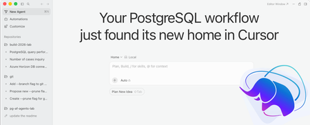
TL; DR: Our Visual Studio Code extension for PostgreSQL is now available on the Open VSX registry: Cursor users get first-class database tooling without leaving the editor that already understands their code. The context switch problem If you use Cursor, you know the feeling. You’re deep in an agentic flow. Composer is scaffolding a feature across multiple files. Tab is anticipating your next move. Then you need to check a table's schema or run a quick query, so you switch to a different tool, and then you lose your flow state, and spend 30 seconds remembering which connection goes to which environment. That context switch is expensive. Not in minutes, but in momentum. Why we built for Cursor (and Open VSX) Cursor is built on the VS Code ecosystem, which means it supports VS Code extensions natively. It uses the Open VSX registry: an open, vendor-neutral extension marketplace where database tooling options have been limited. We saw an opportunity: bring a modern PostgreSQL extension directly to where developers do their most productive work. By publishing to Open VSX, we make sure that developers across the entire VS Code-compatible ecosystem, including Cursor, Windsurf, AWS Kiro, Theia, and Ona all have access without workarounds. Where AI-powered editing meets database awareness Here’s what gets interesting. Cursor indexes your entire codebase semantically. It knows your Drizzle schemas, your raw SQL files, and your migration directories. Our extension completes the picture by giving the editor a live connection to the actual database. Here’s where they intersect: Schema explorer in your sidebar: browse tables, columns, indexes, and functions without leaving the editor. When Cursor’s agent asks “what columns does the users table have?”, the answer is already visible. Screenshot: Object Explorer sidebar showing tables, columns, and indexes expanded Connection-aware IntelliSense: autocomplete table names, column names, and functions based on your live database schema. This pairs naturally with Cursor’s Tab completions: the AI writes the application logic, and IntelliSense validates the SQL. Inline EXPLAIN diagnostics: catch performance issues before they ship. Write a query and see whether it uses an index or triggers a sequential scan, all without running a separate tool. Zero-config connection discovery: we detect .env files, docker-compose.yml, and ORM connection strings in your project. Your database connection follows your workspace, not a global settings file buried three menus deep. Result export and inline execution: select SQL, run it, and see results in a clean panel. Export to JSON or CSV when you need to share findings with your team. Features that make Cursor + PostgreSQL even better Beyond the basics, the extension includes capabilities that pair especially well with AI-powered workflows: MCP server for AI assistants: the extension registers a Model Context Protocol (MCP) server, so Cursor’s agent can discover and interact with your PostgreSQL databases directly through a standardized tool interface. Ask your AI assistant to inspect a table, run a diagnostic query, or analyze a plan: it has the tools to do it. Agent Mode database tools: dedicated DBAgent MCP tools give AI assistants richer database-analysis capabilities, from schema introspection to performance diagnostics and instruction management. Query plan visualization: explore EXPLAIN output in four synchronized views: an interactive node graph, icicle chart, sortable table, and raw source. Color-coded severity groups expose bottlenecks at a glance, and AI-assisted analysis provides optimization suggestions. Performance dashboard: investigate database performance with DB load charts, query activity, wait-event analysis, session health, and blocking chains. Use natural language to inspect trends, identify bottlenecks, and generate diagnostic SQL. Object Explorer search: find database objects by name without expanding the tree. Search across connections, databases, and schemas. Filter by object type or schema name and navigate directly to any result. Schema-aware “New Query”: right-click a schema in Object Explorer to open a new query with the appropriate search_path already set. No more manual SET search_path before writing queries. Multi-source connection profiles: save connection profiles to your user settings, workspace, or folder. Check workspace profiles into source control so every team member gets the right database connections when they open the project. SSH tunneling built in: connect to databases on private networks through SSH tunnels configured directly in the connection dialog, with ssh-agent support for private key authentication. Built for how you actually work Modern development means ephemeral environments, branch-specific databases, and containers everywhere. The extension is designed around this reality: Automatic detection of PostgreSQL instances running in Docker Project-scoped connections that travel with your workspace Support for standard PostgreSQL connections Integration with both local and cloud versions of PostgreSQL from multiple vendors, and first-class support for Azure Database for PostgreSQL and Azure HorizonDB, with provisioning, backup management, and network configuration: all without leaving the editor. Status bar indicator showing your active database at a glance Get started Install from the Open VSX Registry: search for it in Cursor’s extension panel or install the .vsix directly. Your existing VS Code workflow carries over unchanged. If you’re already using Cursor for its agentic capabilities, adding database awareness to the editor means fewer tabs, fewer context switches, and a tighter feedback loop between your application code and the data layer underneath it. Available now on Open VSX. Works with Cursor, Antigravity, and all the VS Code compatible editors.2.5KViews4likes0CommentsSELECT * FROM build2026_sessions WHERE postgres = true;
Microsoft Build 2026 is around the corner, and this year it’s shaping up to be a big one for PostgreSQL experts and enthusiasts. If you’re a developer working with Postgres, or just love exploring new database technology, there's plenty to get excited about. Microsoft’s new cloud-first evolution of PostgreSQL, Azure HorizonDB, alongside sessions featuring Azure Database for PostgreSQL, will highlight how Postgres is powering the next wave of AI-driven applications. A new horizon in Postgres Build 2026 arrives at a time when the role of databases in modern apps is evolving rapidly. From enabling AI model integration to scaling seamlessly across the cloud, PostgreSQL developers today are dealing with more complex demands than ever. That’s why Azure HorizonDB – Microsoft’s new cloud-native PostgreSQL service – is generating so much buzz ahead of Build. What is Azure HorizonDB? In short, it’s a reimagined version of PostgreSQL designed for cloud-scale performance and AI-era workloads. Azure HorizonDB, introduces a distributed architecture that decouples compute and storage, delivering sub-millisecond latencies and three times the throughput of self-managed Postgres at massive scale. It aims to preserve Postgres’s beloved features and SQL ecosystem while adding next-generation capabilities: built-in vector indexing for high-speed AI/ML retrieval, the ability to run AI models and vector operations directly in the database, and multi-zone replication for resilience. For Postgres developers, this means less time stitching together external data stores or machine learning services – and more time building powerful apps on a unified platform that’s both familiar and built for the future. The bottom line: Microsoft Build 2026 is an ideal opportunity for developers to see Azure HorizonDB in action, learn best practices for modern PostgreSQL architectures, and understand how to leverage Postgres in new scenarios like generative AI and multi-agent applications. Read on for a rundown of sessions covering these topics, complete with what you’ll learn from each one. Top sessions for PostgreSQL databases on Azure Below are key sessions tailored for PostgreSQL users and those interested in Azure HorizonDB, with session types and highlights of what you’ll gain by attending. 🎤 Breakout: From Rows to Reasoning: Designing Databases for AI Apps and Agents (BRK223, 45 min, in-person and digital options) Discover how to architect databases that can power tomorrow’s intelligent applications. This technical breakout will show how AI-ready databases can move beyond plain transactions. You’ll see live demos of integrating transactional, analytical, and vector data in one unified platform, with Azure’s new database capabilities, including Azure HorizonDB. Learn how to simplify your stack by eliminating separate analytics engines or vector stores. The session will highlight patterns that reduce data movement and latency so your apps can efficiently reason over live data with minimal complexity. 🧪 Hands-on lab: Create Advanced Postgres-Powered Agentic Apps with Azure HorizonDB (LAB511, 75 min, in person and digital options) Roll up your sleeves and get hands-on building a real multi-agent AI application with Postgres. In this advanced lab, you’ll create a production-ready AI agent powered by Azure HorizonDB as an all-in-one data, search, and intelligence layer. Experiment with retrieval-augmented generation (RAG) by combining semantic vector search (DiskANN) with traditional SQL queries right inside the database. Implement hybrid search and agent workflows without resorting to external vector databases or glue code – thanks to HorizonDB’s built-in vector indexing and in-database AI model capabilities. This lab is perfect for developers who want to experience how HorizonDB can simplify your stack and boost performance for AI-driven apps. Multiple hands-on labs are offered to suite your schedule. 💻 Demo: Simplify App Dev with Cloud-Native PostgreSQL in Azure HorizonDB (DEM364, 25 min, in-person and digital options) See how to cut your development time and complexity with built-in AI and search features in Postgres. This fast-paced demo shows how Azure HorizonDB helps eliminate the need for separate search engines and AI services by pulling those capabilities straight into PostgreSQL. Expect to learn how you can run hybrid vector + keyword queries using SQL, integrate AI models directly from within the database, and apply full-text search (BM25) and semantic ranking to get smarter results. If you’re eager to deliver intelligent apps faster, with fewer moving parts, this session will show how HorizonDB simplifies your architecture without sacrificing performance. ⚡Lightning Talk: Cloud-Native PostgreSQL, Rebuilt for Scale: Azure HorizonDB (LTG413, 15 min, in-person only) Get a rapid-fire introduction to the architecture behind HorizonDB’s eye-popping performance. This short talk dives into how HorizonDB re-architects core PostgreSQL to deliver effortless scale out and blazing speed. Learn how decoupled compute and storage, predictive caching, and multi-region replication combine to achieve sub-millisecond query latencies and 3× higher throughput than standard Postgres. If you care about performance tuning and high-scale database design, don’t miss this quick primer on the tech under HorizonDB’s hood. 👥 Interactive Table Talk: Scaling PostgreSQL for AI Apps: Patterns and Tradeoffs (TT622, 45 min, in-person only) Bring your questions and ideas to this collaborative discussion. In this open round-table session with community and Microsoft experts, you’ll explore architecture patterns for scaling PostgreSQL to meet the demands of agent-based and AI-driven applications. Discuss real-world strategies for handling vector embeddings in Postgres, unifying relational and document data, integrating with AI models, and more. Compare the trade-offs between different scaling approaches – from monolithic to microservices, sharding strategies, and new technologies like HorizonDB – and learn where each design shines or struggles in production. Come ready to share your experiences and learn from others in the room. ▶️ On-Demand: Smarter PostgreSQL Migrations to Power Modern, Intelligent Apps (OD822, 30 min, digital only) Planning to migrate to Postgres or move your databases to Azure? Start here. This on-demand session focuses on new tools and proven strategies to migrate large-scale databases to Azure Database for PostgreSQL quickly and safely. You’ll see AI-assisted migration tools in action that minimize downtime and risk when moving terabytes of data. Just as importantly, you’ll learn how migrating to Azure unlocks advanced capabilities – from boosted performance and enhanced security to AI-ready features – helping you turn your newly migrated data into intelligent apps and services. On-demand session will be available to stream on the first day of Build. Meet the team: PostgreSQL expert meetups If you’re attending Build in person, stop by the Expert Meetup (EMU) area and head to the relational cloud databases booth. This is your chance to talk directly with the engineers and product teams behind PostgreSQL on Azure. Bring your questions about architecture decisions, scaling patterns, migrations, AI workloads, or anything else on your mind. Whether you want to sanity-check a design, dig deeper into something you saw in a session, or give direct feedback, the EMU space is designed for exactly that convo. How to get the most out of Build (and what to do next) With so much great content lined up, how do you decide where to start? It really depends on what you’re most excited about: Curious about AI and agentic apps: Start with From Rows to Reasoning, then go deeper with the Simplify App Dev with HorizonDB demo or get hands-on at the Azure HorizonDB labs to see how these ideas work in practice. Performance and scale are your focus: The short Lightning Talk on HorizonDB’s cloud-native architecture and the Table Talk on scaling Postgres will both provide unique insights and pro tips for running Postgres at massive scale. Planning a migration to PostgreSQL on Azure: Watch the Smarter PostgreSQL Migrations on-demand session to learn how to migrate large workloads with minimal downtime, and the benefits you can unlock after moving to Azure. Looking for real answers to your specific questions: Make time for the PostgreSQL Expert Meetup area to connect directly with the team. No matter which sessions you choose, Build 2026 promises to be an exciting event for the PostgreSQL developer community. Browse the session catalog, save the sessions that match your interests, and we’ll see you at Build.908Views2likes0Comments
Why do I see many VDI_CLIENT_WORKER sessions in Azure SQL Database — and do they impact performance?
Sometimes you’ll notice many sessions showing the command VDI_CLIENT_WORKER in Azure SQL Database—often around scaling, replica/copy workflows, or internal seeding operations. These sessions can look alarming, especially during a performance investigation, but they are typically internal background workers. This post explains how to recognize them, what’s safe to do (and what isn’t), and how to focus on the real bottlenecks like blocking/deadlocks or log rate throttling when you’re troubleshooting slowness. Why you might see VDI_CLIENT_WORKER sessions in Azure SQL Database The symptom You run a session query (for example, using sys.dm_exec_requests or a monitoring tool) and observe: Many sessions with command text VDI_CLIENT_WORKER They may appear to be “stuck,” persist longer than expected, and can’t be killed Teams may worry these sessions are “the cause” of slowness Why it shows up in Azure SQL In Azure SQL, VDI_CLIENT_* wait types and VDI_CLIENT_WORKER sessions are commonly associated with platform operations that involve copying/seeding—for example: Scaling operations (service objective changes) Geo-replication / copy workflows Replica seeding-like behaviors Important: The presence of these sessions does not automatically mean they are the bottleneck. How to validate whether VDI_CLIENT_WORKER is benign? 1) Correlate to recent platform operations. Ask: did you recently perform (or did the platform perform) one of these? Scale up/down. Creation of replicas / geo-secondary operations. Any database copy-like workflow. If yes, it’s a strong indicator you’re seeing background workers tied to that lifecycle event. 2) Check whether they consume resources. A practical approach: Look for CPU/IO/log pressure at the database level. Compare the timing of slowness reports with spikes in waits/locks/log write percentage. If these sessions show minimal resource consumption and are just “present,” treat them as background noise while you investigate real contention. 3) Don’t try to kill them! These sessions are typically system/internal. Attempts to kill them may fail or be ineffective—and generally aren’t recommended. 4) If you need them to disappear. In many cases, these internal workers naturally age out. If they remain visible and you need a cleanup path, operational actions like failover/restart may clear stale workers (use change control / maintenance windows as appropriate for your environment). (This is a practical operational observation; always weigh downtime/impact.) When performance is actually slow: focus on what usually hurts. In many real-world incidents, the main causes of slowness are: Blocking chains / deadlocks. Transaction log rate throttling (LOG_RATE_GOVERNOR) during heavy DML. Hot queries running concurrently and contending on the same objects. Key takeaways Seeing many VDI_CLIENT_WORKER sessions is often expected around platform copy/seeding workflows and doesn’t automatically indicate a bottleneck. Don’t attempt to kill system/internal workers; instead, validate resource impact and focus on actual bottlenecks. For real slowness, prioritize diagnosing blocking/deadlocks and LOG_RATE_GOVERNOR-driven DML throttling.170Views0likes0Comments