performance
581 TopicsSystem Windows Ram Problem Fix
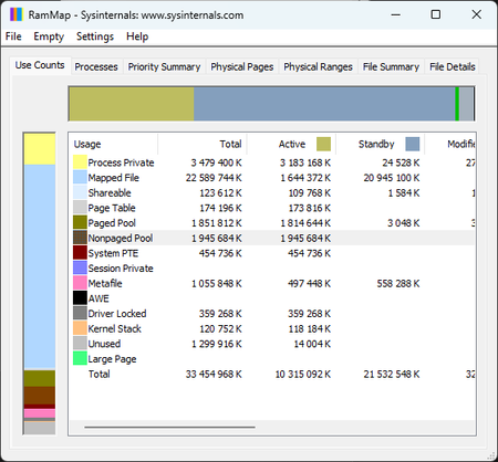
You’ve probably seen this happen — you leave your desktop or laptop running, and after a while the system starts eating a huge chunk of your RAM, even on modern hardware. Today I’m bringing a fix that removes this issue permanently and gives Windows back the speed, stability, and clean behavior it should have. By disabling two legacy predictive mechanisms (SysMain + Prefetch), the system stops aggressively caching applications, idle RAM usage drops significantly, and micro‑lags disappear. The attached screenshots show the system before and after applying the fix. This solution works on both Windows 10 and Windows 11, and it’s safe, reversible, and the improvement is immediate. System Ram Before: System Ram After: Step‑by‑step guide (Windows 10 / 11 RAM issue fix) Note: This is a safe and fully reversible system tweak. You’re simply disabling two legacy predictive mechanisms that no longer make sense on modern hardware. 1️⃣ Disable the SysMain service Press Win + R Type services.msc → press Enter Find SysMain in the list Double‑click it Set Startup type to Disabled Click Stop if the service is running Confirm with Apply and OK 2️⃣ Disable Prefetch in the Registry Press Win + R Type regedit → press Enter Navigate to: HKEY_LOCAL_MACHINE\SYSTEM\CurrentControlSet\Control\Session Manager\Memory Management\PrefetchParameters Find the value EnablePrefetcher Double‑click it and set the value to: 0 Confirm with OK 3️⃣ Restart your system After rebooting, your RAM usage in idle should drop noticeably, and the system will feel cleaner, faster, and more responsive. 4️⃣ How to revert (optional) If you ever want to undo the changes: SysMain: set Startup type back to Automatic and start the service EnablePrefetcher: set the value back to 3 (default) With my regular applications open, RAM usage dropped from 60–70% to just 33%. This is how Windows should have behaved from the beginning. On top of that, overall system responsiveness improved by roughly 50% — even weaker hardware feels noticeably faster almost immediately. This RAM regression has been around since Windows 7. After the kernel overhaul in Windows 8.1 it actually got worse, and it has followed every version of Windows all the way to today. RAM stability after - optimization results: RAM stability after 21 hours uptime – optimization results | Microsoft Community Hub2.6KViews0likes3CommentsEngineering Agentic Recall Controls with MCP and Microsoft Foundry
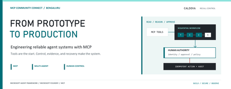
AI agents become operationally interesting when they can reach real systems. They also become operationally dangerous at exactly the same moment. Caldova Recall Control Tower is a developer demonstration built around that tension. It uses a fictional pharmaceutical recall to show how an agent can gather evidence and prepare a decision while deterministic application code retains authority over approval and inventory mutation. The implementation combines the Model Context Protocol (MCP), Microsoft Agent Framework, a Microsoft Foundry Hosted Agent, FastAPI, Microsoft Entra authentication, managed identity, and optimistic concurrency in Azure Blob Storage. Central design rule: Let the model interpret and recommend. Make ordinary code authenticate, authorize, mutate, and prove what happened. Caldova is fictional, all operational data is synthetic, and this sample is not a production recall system or a source of clinical advice. The scenario: useful reasoning, consequential action The demo starts with a temperature excursion affecting batch B-2408-AX7 of Caldova Relief 20 mg tablets. The synthetic inventory contains 2,196 units across two distribution centers and two retail stores. A useful system must establish the notice, locate every affected position, check supplier status, explain uncertainty, and recommend an action. That analysis is a good fit for specialized agents. Quarantining inventory is not. Quarantine changes operational state. It therefore needs an authenticated human, explicit authorization, a batch-scoped approval, concurrency control, idempotency, and an audit record. None of those guarantees should depend on a prompt being followed. The authenticated hosted application at the start of the fictional recall. Architecture: separate reasoning from authority The solution has two related but deliberately separate paths. Caldova separates model reasoning from application authority. Official Microsoft service icons identify Foundry Agent Service, App Service, Managed Identity, and Blob Storage. The reasoning path invokes a Hosted Agent through the Responses protocol. Four agents run in a fixed sequence: triage, inventory impact, supplier/compliance, and supervisor. The first three have narrow read-only tools. The supervisor has no tools and synthesizes the accumulated context into a decision brief. The authority path remains in the web application. It validates the EasyAuth identity claims, checks an approver allowlist, binds approval to the caller, batch, action, and current demo generation, and only then calls deterministic domain code. State is stored per actor in Blob Storage and updated with ETag match conditions so concurrent writes fail instead of silently overwriting each other. There is also a deterministic localhost demo. It reuses synthetic domain fixtures and demonstrates MCP contracts, approval, quarantine, and replay without a model or cloud account. It is useful for development, but its typed approver name and in-memory state are not production identity or durable compliance evidence. Building a narrow MCP surface MCP standardizes how an AI application discovers and calls external tools. It does not remove the need to design those tools carefully. Caldova exposes small, typed operations such as get_recall_notice , locate_inventory , and get_supplier_status . Inputs are constrained with Pydantic, and tool annotations tell clients that these operations are read-only and closed-world: @mcp.tool( title="Locate affected inventory", annotations=ToolAnnotations( read_only_hint=True, open_world_hint=False, ), ) def locate_inventory(batch_id: BatchId) -> dict[str, Any]: return STORE.locate_inventory(batch_id) The mutation tool is separately marked destructive and requires a batch-scoped approval token. Those annotations improve discovery and planning, but they are metadata, not an authorization boundary. The real check occurs inside quarantine_batch , below the model and below the tool description. The Hosted Agent does not receive the mutation tools at all. Its specialists call only three read operations through an isolated MCP stdio subprocess. This is stronger than asking an all-powerful agent to "please remain read-only": capability is constrained by construction. The subprocess boundary also keeps MCP v2 dependencies isolated from the Foundry hosting environment. Each call has a timeout, bounded concurrency, structured JSON handling, and a generic failure response that does not leak subprocess details. Fixed workflows beat vague autonomy for this case Multi-agent does not have to mean dynamic routing. Caldova uses an explicit sequence because the business dependency is explicit: validate the notice before locating inventory, locate inventory before checking supplier implications, and synthesize only after all three specialist outputs exist. return ( WorkflowBuilder(start_executor=triage, output_from=[supervisor]) .add_edge(triage, inventory) .add_edge(inventory, compliance) .add_edge(compliance, supervisor) .build() .as_agent() ) This topology is easier to test and reason about than an unconstrained planner. Each specialist has one job and one tool allowlist. Full context is passed where synthesis requires it, while the supervisor remains tool-free. Request isolation matters too. A hosted process can serve concurrent users, so workflow state must not leak between requests. The sample creates a fresh workflow agent for each request context rather than reusing mutable agent state globally. What the live hosted run showed The hosted application completed a read-only assessment for the synthetic batch. The resulting brief reported: 2,196 affected units across four locations. A high-risk inbound temperature excursion. Supplier acknowledgement, a 36-hour replacement estimate, and a drafted credit note. Unknown transit temperature details, excursion duration, stability impact, final supplier disposition, and potentially issued stock. A recommendation to hold or quarantine stock, explicitly stating that no quarantine had occurred. A required human approval before any inventory restriction. The live Hosted Agent decision brief. Transient response and correlation identifiers are masked; the operations rail is excluded because it contains actor-scoped audit data. The screenshot also shows an important truthfulness choice: the UI says Hosted workflow trace unavailable. The application does not invent stage completion or tool-call evidence when the hosted endpoint does not return trustworthy trace data. The answer can be displayed, but it must not be presented as proof of an internal execution path. Approval is a protocol, not a button The hosted web path uses App Service authentication with Microsoft Entra. The application accepts the injected principal only on the configured App Service host, validates tenant and object identifiers, applies a user allowlist, and performs an additional approver check for mutation requests. State-changing calls also require the expected origin and an application request header. Approval is then bound to five facts: The authenticated actor. The current demo generation. The affected batch. The quarantine action. A ten-minute validity window until first use. Resetting the demo creates a new generation, invalidating old handles. Consuming an approval does not make replay unsafe: the same bound handle can repeat the same quarantine operation, but domain code changes only positions that are not already quarantined. A second call reports an idempotent replay with zero additional positions changed. This is the difference between a human-in-the-loop interface and a human-authorized system. A modal dialog provides user experience; identity binding and deterministic policy provide control. Durable state needs concurrency semantics The hosted application stores each actor's synthetic session in a separate Blob object. A load returns both JSON state and its ETag. A save uses IfNotModified semantics; if another request updated the same state first, Azure Storage rejects the stale write and the API returns a conflict. conditions = ( {"etag": etag, "match_condition": MatchConditions.IfNotModified} if etag else {} ) await blob.upload_blob( json.dumps(state), overwrite=etag is not None, **conditions, ) Without that condition, two browser requests could both read the same approval state and overwrite one another using last-writer-wins behavior. Agent systems do not get a concurrency exemption: ordinary distributed-systems rules still apply. Fail closed, and make the failure legible The analysis adapter accepts only HTTPS Foundry endpoints with the expected path, uses a managed-identity token for https://ai.azure.com/.default , disables redirects, and enforces bounded connect and overall timeouts. It accepts only a completed assistant response with non-empty output text. If the endpoint times out, returns partial output, returns malformed data, or becomes unavailable, the application clears the analysis lease and reports that no inventory changed. It does not substitute a local answer and label it as hosted. Approval remains locked until a new hosted analysis succeeds. This can feel strict during a demo, but it protects provenance. A degraded fallback is useful only when the UI and audit model can identify it accurately. What is proven, and what is not The sample provides useful evidence for several engineering claims: Typed MCP tools reject malformed input. Hosted specialists receive read-only capabilities only. Approval is checked below the model and bound to identity and session state. Quarantine is idempotent in the synthetic domain. Blob ETags prevent stale session writes. Empty, partial, failed, and timed-out hosted responses fail closed. Local tests cover domain, MCP, workflow, API, and repository-hygiene behavior. It does not prove that the sample is a production recall platform. The scenario is synthetic. The local audit log is not tamper-evident. The hosted UI currently lacks trustworthy per-stage and per-tool trace rendering. Deployment-specific RBAC, EasyAuth configuration, telemetry access, model behavior, load characteristics, costs, and recovery procedures require validation in each environment. Evaluation evidence also expires. Golden cases and evaluator configuration are useful assets, but historical results are not a current release certificate. Re-run evaluations against the deployed agent version and inspect failures before making quality claims. Try the pattern Start with the deterministic path before provisioning cloud resources: Set-Location (git rev-parse --show-toplevel) py -3.13 -m venv caldova-recall-control/.venv ./caldova-recall-control/.venv/Scripts/python.exe -m pip install ` -r caldova-recall-control/requirements-ui.txt ./caldova-recall-control/.venv/Scripts/python.exe -m uvicorn ` control_tower_api:app ` --app-dir caldova-recall-control/src ` --host 127.0.0.1 ` --port 8091 Then inspect the MCP server over stdio: ./caldova-recall-control/.venv/Scripts/python.exe ` caldova-recall-control/scripts/inspect_mcp.py The inspector discovers the real tool schemas, reads the synthetic inventory, rejects malformed input and an unapproved mutation, and confirms the stock remains unchanged. Only after that local contract is understood should you configure a Foundry project, deployment identity, model deployment, and Hosted Agent. Engineering takeaways The most reusable lesson in Caldova is not the number of agents. It is the placement of authority. Give each model the smallest useful toolset. Prefer explicit workflow topology when the business process is known. Treat tool annotations as descriptive metadata, not access control. Bind consequential approval to authenticated identity, resource, action, and session generation. Put mutation and idempotency in deterministic domain code. Use optimistic concurrency for durable web state. Preserve provenance by failing closed instead of silently changing execution paths. Show only evidence the system actually captured. Agents are excellent at turning fragmented evidence into an actionable brief. Reliable systems make sure the brief and the action remain two different things. References Caldova source repository Model Context Protocol introduction Microsoft Agent Framework workflow capabilities Deploy a Hosted Agent in Microsoft Foundry Configure Microsoft Entra authentication for Azure App Service Manage concurrency in Azure Blob StorageGeneric Best Practices for HikariCP with Azure Database for PostgreSQL
Author: Mohamed Baioumy Technology: Azure Database for PostgreSQL (Flexible Server & Single Server) Category: Connectivity | Performance | Application Design Introduction Connection pooling is a critical component of application performance when connecting to Azure Database for PostgreSQL. Creating a new PostgreSQL connection is an expensive operation that consumes CPU, memory, and networking resources. Reusing existing connections through a connection pool significantly reduces connection latency, improves throughput, and helps applications scale more efficiently. Many Java applications use HikariCP, one of the most popular high-performance JDBC connection pools. While HikariCP provides excellent performance out of the box, improperly configured connection pool settings can lead to issues such as: Connection pool exhaustion Stale or invalid connections Increased connection acquisition latency Excessive connection creation and destruction Database resource contention Application timeouts This article summarizes generic guidance and best practices for configuring HikariCP when working with Azure Database for PostgreSQL Flexible Server and Azure Database for PostgreSQL Single Server. Understanding Key HikariCP Parameters 1. Maximum Lifetime (maxLifetime) The maxLifetime property controls how long a connection can remain in the pool before HikariCP retires it and creates a new one. Why It Matters Connections can become stale over time due to: Network interruptions Infrastructure updates Connection state changes TCP idle behavior Recycling connections periodically helps prevent applications from using long-lived connections that may no longer be healthy. Recommended Practice Avoid configuring the value too low. When maxLifetime is set aggressively, HikariCP continuously destroys and recreates connections, resulting in: Additional authentication overhead Increased connection establishment latency Higher CPU utilization Reduced application throughput A reasonable starting point is: spring.datasource.hikari.maxLifetime=1800000 30 minutes (1,800,000 ms) is commonly used and aligns well with many production workloads. Depending on workload characteristics, values between 30 minutes and 1 hour are generally suitable Avoid maxLifetime=300000 (5 minutes) This often causes unnecessary connection churn without providing additional benefits. 2. Minimum Idle Connections (minimumIdle) The minimumIdle setting defines how many idle connections HikariCP should keep ready for immediate use. Why It Matters A pool with available idle connections can serve application requests immediately without waiting for new connections to be established. However, maintaining too many idle connections consumes unnecessary database resources. Recommended Practice For most workloads: minimumIdle = maximumPoolSize Or minimumIdle slightly lower than maximumPoolSize This ensures sufficient connections are already available during traffic spikes while avoiding excessive connection creation delays. Example maximumPoolSize=20 minimumIdle=15 Avoid maximumPoolSize=20 minimumIdle=20 only when the application experiences long periods of inactivity and conserving resources is more important than immediate responsiveness. 3. Idle Timeout (idleTimeout) The idleTimeout property determines how long an unused connection remains in the pool before being removed. Why It Matters Connections that sit idle for extended periods consume resources on both: The application server Azure Database for PostgreSQL However, removing idle connections too quickly causes the application to repeatedly establish new connections. Recommended Practice Keep the default value unless there is a specific requirement. spring.datasource.hikari.idleTimeout=600000 which equals: 10 minutes (600,000 ms) This setting provides a good balance between resource utilization and responsiveness. [Re: EXT: R...0040002947 | Outlook] The timeout should also be comfortably longer than any expected short application idle periods. Avoid idleTimeout=10000 (10 seconds) Such aggressive settings often result in unnecessary connection creation cycles. 4. Maximum Pool Size (maximumPoolSize) This parameter determines the maximum number of concurrent database connections the application can maintain. Why It Matters This is often the most important HikariCP setting. If the Pool Is Too Small Applications may experience: Connection is not available, request timed out because all available connections are already in use. Similar scenarios have been observed during customer investigations involving Hikari pool exhaustion. If the Pool Is Too Large Applications can overwhelm the database server with excessive concurrent sessions, resulting in: Connection contention Increased context switching Higher memory consumption Reduced overall performance Recommended Practice Pool size should be based on: Database compute configuration CPU core count Query execution duration Application concurrency requirements Workload characteristics There is no universal value that fits every workload. Start conservatively: maximumPoolSize=10 or maximumPoolSize=20 maximumPoolSize=20 and increase only after load testing demonstrates a need for additional concurrency. Fixed-Size Pool Recommendation For many production workloads, a fixed-size pool provides the simplest and most predictable behavior. Configure: maximumPoolSize=20 minimumIdle=20 or omit minimumIdle entirely so it defaults to maximumPoolSize. HikariCP commonly recommends maintaining a fixed-size pool for responsiveness during demand spikes. Benefits Faster connection acquisition Predictable performance Reduced connection creation latency Better handling of traffic spikes When using a small fixed-size pool, there is often little need to aggressively tune: minimumIdle idleTimeout Instead, simply recycle connections using: maxLifetime maxLifetime Additional Recommendations Enable TCP Keepalive One common cause of stale connections is network devices silently dropping inactive TCP sessions. For PostgreSQL applications, consider enabling TCP keepalive: tcpKeepAlive=true tcpKeepAlive=true The HikariCP project specifically recommends enabling TCP keepalive to prevent rare situations where pools can lose valid connections. Monitor Connection Usage Track: Active connections Idle connections Connection acquisition time Pool exhaustion events Database connection counts These metrics help identify whether pool sizing is appropriate. Investigate Long-Running Queries Connection pool problems are often symptoms rather than root causes. A frequent scenario is: A query becomes slow. Connections remain occupied longer. The pool becomes exhausted. Applications start timing out. When analyzing HikariCP issues, always review: Query performance Blocking situations Database resource utilization Application connection handling logic Sample Production Configuration spring.datasource.hikari.maximumPoolSize=20 spring.datasource.hikari.minimumIdle=15 spring.datasource.hikari.maxLifetime=1800000 spring.datasource.hikari.idleTimeout=600000 spring.datasource.hikari.connectionTimeout=30000 spring.datasource.hikari.keepaliveTime=60000 spring.datasource.hikari.maximumPoolSize=20 spring.datasource.hikari.minimumIdle=15 spring.datasource.hikari.maxLifetime=1800000 spring.datasource.hikari.idleTimeout=600000 spring.datasource.hikari.connectionTimeout=30000 spring.datasource.hikari.keepaliveTime=60000 This configuration provides a solid starting point for many Azure Database for PostgreSQL workloads and can be adjusted based on application-specific requirements. a { text-decoration: none; color: #464feb; } tr th, tr td { border: 1px solid #e6e6e6; } tr th { background-color: #f5f5f5; } Conclusion HikariCP is extremely efficient when configured appropriately. The goal is not to maximize the number of connections, but rather to maintain a healthy balance between application responsiveness and database resource consumption. As a general rule: Use a reasonable maxLifetime (30–60 minutes) Keep enough idle connections available for traffic spikes Avoid aggressive idleTimeout values Size the pool based on workload characteristics, not guesses Consider fixed-size pools for predictable performance Monitor connection usage and query performance regularly By following these practices, applications connecting to Azure Database for PostgreSQL can achieve improved scalability, lower latency, and more reliable connectivity. References Connection pooling best practices - Azure Database for PostgreSQL Performance best practices for using Azure Database for PostgreSQL – Connection Pooling HikariCP Documentation and Pool Sizing GuidanceLessons Learned #540:Bulk Insert Throughput in Azure SQL Hyperscale with Partitioned Heap Tables
In this lesson learned, I would like to share an interesting scenario working on a service request where our customer was running a high-volume data load process in Azure SQL Database Hyperscale. The workload was based on a common pattern: Recreate a staging table. Load a large number of rows using bulk insert. The bulk insert showed unstable execution times and became the main area to investigate. The process was loading a very large number of rows into an Azure SQL Database Hyperscale database. The process used a staging table that was initially loaded as a heap. The main concern was the inconsistent execution time during the load process. Why Manually Adding Data Files Was Not the Right Direction In Azure SQL Database Hyperscale, the storage architecture is different from a traditional SQL Server deployment. The data layout and storage management are handled internally by the service. Because of this architecture, manually creating or pre-allocating multiple data files is not the same tuning option that we may consider in SQL Server on-premises or SQL Server running on Azure Virtual Machines. For this reason, the troubleshooting focus moved from manual file layout configuration to the actual workload pattern, waits, concurrency, batch size, and staging table design. What We Observed During the bulk insert phase, waits such as PAGELATCH_EX were observed. Since the staging table was loaded as a heap and the clustered primary key was created only after the bulk insert completed, OPTIMIZE_FOR_SEQUENTIAL_KEY was not directly applicable to the bulk insert phase. This changed the direction of the investigation. Instead of focusing on last-page insert contention on an existing clustered index, the analysis moved toward heap insert behavior, allocation contention, concurrency, batch size, and whether a different staging table design could help. First Recommendation: Start with Low-Impact Changes Before changing the table design, the first recommendation was to test the least intrusive changes: Reduce the number of concurrent bulk insert sessions. Increase the batch size, for example from 10,000 rows to 50,000 or 100,000 rows. Test TABLOCK on the dedicated heap staging table. The goal was to avoid assuming that more concurrency would always reduce the total execution time. In some high-volume load scenarios, excessive concurrency may increase contention and make the process less stable. The Interesting Design Option: Partitioned Heap Staging Table One of the most interesting design options was to evaluate a partitioned heap staging table. The idea is simple: instead of loading all rows into a non-partitioned heap staging table, the staging table can be created on the same partition scheme used by the target table, using the same partitioning column. This does not mean that a partitioned heap will always be faster. However, it can be a useful design option when: The bulk load phase is affected by allocation or latch contention. Concurrent load processes can naturally distribute rows across different partition ranges. The staging table is used only as an intermediate structure.Lessons Learned The main lessons from this scenario were: In Azure SQL Database Hyperscale, manually managing multiple data files is not the right tuning direction. PAGELATCH_EX during heap loading may point to concurrency or allocation-related contention. Reducing concurrency can sometimes improve total throughput. Larger batch sizes may provide better results than many small batches. TABLOCK on a dedicated heap staging table is a low-impact test worth evaluating. A partitioned heap staging table can be a valid second-phase design option when the load can be distributed across partition ranges. The best approach is to test small, measurable changes before introducing architectural redesigns. Final Thoughts A partitioned heap staging table can be a powerful option, but only when it is tested carefully and when the workload pattern can benefit from partition distribution.224Views0likes0CommentsDistributing Agents to Microsoft Teams and Microsoft 365 Copilot Part 4/5
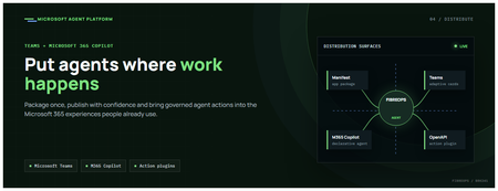
This is the fourth post in our series on the Microsoft agent platform. We cover the Distribute in M365 pillar — publishing your agents to Microsoft Teams and Microsoft 365 Copilot so they reach users where they already work. All examples reference the FibreOps repository, demonstrated at Microsoft Build BRK241. The Distribution Story Building a great agent is only half the challenge. The other half is getting it into the hands of users without asking them to learn a new tool, visit a new URL, or change their workflow. Microsoft 365 Copilot and Microsoft Teams are where enterprise users already spend their day, making them the natural distribution surface for agents. With the GA release, publishing an agent to Teams and M365 Copilot is a single command. No separate app registration portal, no manual manifest assembly, no multi-step approval workflow for development and testing. Publishing to Microsoft 365 Copilot (GA) FibreOps ships as a declarative agent + action plugin ready for sideload. A single CLI command produces the complete package: python -m fibreops.demo publish-m365 --out dist/m365 # Output: # ✓ wrote dist/m365/declarativeAgent.json # ✓ wrote dist/m365/fibreops-action.json # ✓ wrote dist/m365/manifest.json # ✓ wrote dist/m365/color.png (192x192) # ✓ wrote dist/m365/outline.png ( 32x32) # ✓ wrote dist/m365/fibreops-copilot.zip What Gets Generated File Purpose declarativeAgent.json Defines the agent's persona, capabilities, and conversation starters for M365 Copilot fibreops-action.json Action plugin that proxies tool calls to the deployed FastAPI backend via OpenAPI manifest.json Teams app manifest with publisher metadata, permissions, and capabilities color.png / outline.png App icons for Teams and M365 surfaces fibreops-copilot.zip Ready-to-upload package for Teams Admin Center Configuration Set the base URL to your deployed FastAPI app before publishing — the action plugin uses this to resolve the OpenAPI runtime: # Set the public HTTPS hostname of the deployed FastAPI app $env:M365_ACTION_BASE_URL = "https://fibreops-demo.azurewebsites.net" # Optional: customise publisher metadata $env:M365_PUBLISHER_NAME = "Contoso Network Operations" $env:M365_PUBLISHER_WEBSITE = "https://contoso.com/noc" # Generate the package python -m fibreops.demo publish-m365 --out dist/m365 Environment Variable Purpose M365_ACTION_BASE_URL Public HTTPS root for the FastAPI /openapi.json (e.g., Container Apps FQDN) M365_APP_ID Override the generated Teams app GUID (default: deterministic per repo) M365_PUBLISHER_NAME Publisher name shown in M365 Admin Center M365_PUBLISHER_WEBSITE Publisher website link Uploading the Package Upload the generated fibreops-copilot.zip through either path: Teams Admin Center → Manage apps → Upload new app M365 Admin Center → Integrated apps → Upload custom apps Once uploaded, the declarative agent: Inherits the publisher metadata you configured Advertises conversation starters from the FibreOps deck (e.g., "What is the current outage status?", "Dispatch an engineer to FN-LDN-001") Proxies tool calls to the deployed FastAPI app via the action plugin Appears in Microsoft 365 Copilot as a specialised agent users can invoke How Declarative Agents Work A declarative agent in Microsoft 365 Copilot is defined by metadata rather than code running in the M365 surface. The intelligence lives in your backend — Copilot handles the conversational UX, tool orchestration schema, and user authentication. The flow: User invokes the agent in Microsoft 365 Copilot or Teams Copilot renders conversation starters and accepts natural language input When the agent needs to act, Copilot calls the action plugin (your OpenAPI endpoint) Your FastAPI backend processes the request using the full agent pipeline Results return to the user in the Copilot/Teams UX This architecture means your agent logic stays in one place — the backend. The M365 surface is purely a distribution and interaction layer. Action Plugins and OpenAPI The action plugin ( fibreops-action.json ) references your FastAPI app's /openapi.json endpoint. FibreOps exposes a JSON API that the action plugin can call: /api/runs — List and query agent runs /api/optimiser — Get optimizer scores and suggestions /sdk/chat — Natural language interaction with the agent system /healthz — Liveness probe Because FastAPI auto-generates OpenAPI schemas from your typed Python endpoints, the action plugin gets accurate parameter descriptions, response schemas, and error codes without any manual specification work. Publishing as Autopilots (Public Preview) Autopilots take distribution one step further — agents that operate autonomously without requiring a user to initiate each interaction. An Autopilot can: React to events (e.g., a critical telemetry signal) without human initiation Take actions within defined guardrails Notify users only when human intervention is needed Operate continuously across Microsoft 365 surfaces For FibreOps, an Autopilot would monitor the Event Hub stream continuously and only surface to the NOC team when an incident exceeds automated resolution capability — a fully autonomous operations agent. Teams Adaptive Cards FibreOps posts rich Adaptive Card notifications to Microsoft Teams throughout the agent pipeline. This is separate from the declarative agent — it is a push notification channel for real-time operational awareness. # The NetOps agent posts an outage notice via Incoming Webhook def post_outage_notice(incident_id, node_id, severity, summary, engineer=None): card = { "type": "AdaptiveCard", "body": [ {"type": "TextBlock", "text": f"🚨 Outage: {node_id}", "weight": "Bolder", "size": "Large"}, {"type": "FactSet", "facts": [ {"title": "Severity", "value": severity.upper()}, {"title": "Incident", "value": incident_id}, {"title": "Summary", "value": summary}, ]}, ], "actions": [ {"type": "Action.OpenUrl", "title": "View in NOC Console", "url": f"{base_url}/runs/{incident_id}"} ] } # POST to Teams webhook or append to outbox for offline mode ... If TEAMS_WEBHOOK_URL is not configured, cards are appended to state/teams_outbox.jsonl for review in the NOC console's Teams panel. End-to-End: From Code to Copilot Here is the complete flow from development to distribution: Build — Develop agents with Microsoft Agent Framework, test locally with python -m fibreops.demo --backend local Publish agents — python -m fibreops.demo publish creates hosted Prompt Agents in Foundry Deploy infrastructure — azd up provisions App Service, ACR, Event Hub, Key Vault, and Application Insights Deploy hosted agent — azd env set FIBREOPS_DEPLOY_HOSTED true && azd up Generate M365 package — python -m fibreops.demo publish-m365 --out dist/m365 Upload to Teams — Upload fibreops-copilot.zip via Teams Admin Center Users interact — The agent is now available in Microsoft 365 Copilot and Teams Security Considerations Managed Identity — The deployed app uses system-assigned managed identity for all Azure service access. No secrets in code. Least privilege — Each role grant is scoped to the minimum required (Event Hubs Data Owner, Key Vault Secrets User, AcrPull, Azure AI Developer). Authentication — The M365 Copilot surface handles user authentication; your backend receives authenticated requests. Guardrails — Autopilots operate within defined boundaries; human-in-the-loop escalation is built into the Routine and agent decision logic. Key Takeaways Publishing to Teams and M365 Copilot is GA — a single command generates the complete package. Declarative agents separate distribution (M365) from intelligence (your backend). Action plugins leverage your existing FastAPI OpenAPI schema — no manual specification needed. Autopilots (Public Preview) enable fully autonomous operation within guardrails. Adaptive Cards provide real-time push notifications alongside the conversational agent surface. The same backend serves the NOC console, the Copilot SDK, and the M365 declarative agent. Next Steps Explore the FibreOps repository — try python -m fibreops.demo publish-m365 Microsoft 365 Copilot extensibility documentation Next in this series: Voice Live and Observability for Production Agent SystemsBuilding HIPAA-Compliant Medical Transcription with Local AI
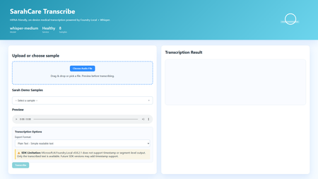
Building HIPAA-Compliant Medical Transcription with Local AI Introduction Healthcare organizations generate vast amounts of spoken content, patient consultations, research interviews, clinical notes, medical conferences. Transcribing these recordings traditionally requires either manual typing (time-consuming and expensive) or cloud transcription services (creating immediate HIPAA compliance concerns). Every audio file sent to external APIs exposes Protected Health Information (PHI), requires Business Associate Agreements, creates audit trails on third-party servers, and introduces potential breach vectors. This sample solution lies in on-premises voice-to-text systems that process audio entirely locally, never sending PHI beyond organizational boundaries. This article demonstrates building a sample medical transcription application using FLWhisper, ASP.NET Core, C#, and Microsoft Foundry Local with OpenAI Whisper models. You'll learn how to build sample HIPAA-compliant audio processing, integrate Whisper models for medical terminology accuracy, design privacy-first API patterns, and build responsive web UIs for healthcare workflows. Whether you're developing electronic health record (EHR) integrations, building clinical research platforms, or implementing dictation systems for medical practices, this sample could be a great starting point for privacy-first speech recognition. Why Local Transcription Is Critical for Healthcare Healthcare data handling is fundamentally different from general business data due to HIPAA regulations, state privacy laws, and professional ethics obligations. Understanding these requirements explains why cloud transcription services, despite their convenience, create unacceptable risks for medical applications. HIPAA compliance mandates strict controls over PHI. Every system that touches patient data must implement administrative, physical, and technical safeguards. Cloud transcription APIs require Business Associate Agreements (BAAs), but even with paperwork, you're entrusting PHI to external systems. Every API call creates logs on vendor servers, potentially in multiple jurisdictions. Data breaches at transcription vendors expose patient information, creating liability for healthcare organizations. On-premises processing eliminates these third-party risks entirely, PHI never leaves your controlled environment. US State laws increasingly add requirements beyond HIPAA. California's CCPA, New York's SHIELD Act, and similar legislation create additional compliance obligations. International regulations like GDPR prohibit transferring health data outside approved jurisdictions. Local processing simplifies compliance by keeping data within organizational boundaries. Research applications face even stricter requirements. Institutional Review Boards (IRBs) often require explicit consent for data sharing with external parties. Cloud transcription may violate study protocols that promise "no third-party data sharing." Clinical trials in pharmaceutical development handle proprietary information alongside PHI, double jeopardy for data exposure. Local transcription maintains research integrity while enabling audio analysis. Cost considerations favor local deployment at scale. Medical organizations generate substantial audio, thousands of patient encounters monthly. Cloud APIs charge per minute of audio, creating significant recurring costs. Local models have fixed infrastructure costs that scale economically. A modest GPU server can process hundreds of hours monthly at predictable expense. Latency matters for clinical workflows. Doctors and nurses need transcriptions available immediately after patient encounters to review and edit while details are fresh. Cloud APIs introduce network delays, especially problematic in rural health facilities with limited connectivity. Local inference provides <1 second turnaround for typical consultation lengths. Application Architecture: ASP.NET Core with Foundry Local The sample FLWhisper application implements clean separation between audio handling, AI inference, and state management using modern .NET patterns: The ASP.NET Core 10 minimal API provides HTTP endpoints for health checks, audio transcription, and sample file streaming. Minimal APIs reduce boilerplate while maintaining full middleware support for error handling, authentication, and CORS. The API design follows OpenAI's transcription endpoint specification, enabling drop-in replacement for existing integrations. The service layer encapsulates business logic: FoundryModelService manages model loading and lifetime, TranscriptionService handles audio processing and AI inference, and SampleAudioService provides demonstration files for testing. This separation enables easy testing, dependency injection, and service swapping. Foundry Local integration uses the Microsoft.AI.Foundry.Local.WinML SDK. Unlike cloud APIs requiring authentication and network calls, this SDK communicates directly with the local Foundry service via in-process calls. Models load once at startup, remaining resident in memory for sub-second inference on subsequent requests. The static file frontend delivers vanilla HTML/CSS/JavaScript, no framework overhead. This simplicity aids healthcare IT security audits and enables deployment on locked-down hospital networks. The UI provides file upload, sample selection, audio preview, transcription requests, and result display with copy-to-clipboard functionality. Here's the architectural flow for transcription requests: Web UI (Upload Audio File) ↓ POST /v1/audio/transcriptions (Multipart Form Data) ↓ ASP.NET Core API Route ↓ TranscriptionService.TranscribeAudio(audioStream) ↓ Foundry Local Model (Whisper Medium locally) ↓ Text Result + Metadata (language, duration) ↓ Return JSON/Text Response ↓ Display in UI This architecture embodies several healthcare system design principles: Data never leaves the device: All processing occurs on-premises, no external API calls No data persistence by default: Audio and transcripts are session-only, never saved unless explicitly configured Comprehensive health checks: System readiness verification before accepting PHI Audit logging support: Structured logging for compliance documentation Graceful degradation: Clear error messages when models unavailable rather than silent failures Setting Up Foundry Local with Whisper Models Foundry Local supports multiple Whisper model sizes, each with different accuracy/speed tradeoffs. For medical transcription, accuracy is paramount—misheard drug names or dosages create patient safety risks: # Install Foundry Local (Windows) winget install Microsoft.FoundryLocal # Verify installation foundry --version # Download Whisper Medium model (optimal for medical accuracy) foundry model add openai-whisper-medium-generic-cpu:1 # Check model availability foundry model list Whisper Medium (769M parameters) provides the best balance for medical use. Smaller models (Tiny, Base) miss medical terminology frequently. Larger models (Large) offer marginal accuracy gains at 3x inference time. Medium handles medical vocabulary well, drug names, anatomical terms, procedure names, while processing typical consultation audio (5-10 minutes) in under 30 seconds. The application detects and loads the model automatically: // Services/FoundryModelService.cs using Microsoft.AI.Foundry.Local.WinML; public class FoundryModelService { private readonly ILogger _logger; private readonly FoundryOptions _options; private ILocalAIModel? _loadedModel; public FoundryModelService( ILogger logger, IOptions options) { _logger = logger; _options = options.Value; } public async Task InitializeModelAsync() { try { _logger.LogInformation( "Loading Foundry model: {ModelAlias}", _options.ModelAlias ); // Load model from Foundry Local _loadedModel = await FoundryClient.LoadModelAsync( modelAlias: _options.ModelAlias, cancellationToken: CancellationToken.None ); if (_loadedModel == null) { _logger.LogWarning("Model loaded but returned null instance"); return false; } _logger.LogInformation( "Successfully loaded model: {ModelAlias}", _options.ModelAlias ); return true; } catch (Exception ex) { _logger.LogError( ex, "Failed to load Foundry model: {ModelAlias}", _options.ModelAlias ); return false; } } public ILocalAIModel? GetLoadedModel() => _loadedModel; public async Task UnloadModelAsync() { if (_loadedModel != null) { await FoundryClient.UnloadModelAsync(_loadedModel); _loadedModel = null; _logger.LogInformation("Model unloaded"); } } } Configuration lives in appsettings.json , enabling easy customization without code changes: { "Foundry": { "ModelAlias": "whisper-medium", "LogLevel": "Information" }, "Transcription": { "MaxAudioDurationSeconds": 300, "SupportedFormats": ["wav", "mp3", "m4a", "flac"], "DefaultLanguage": "en" } } Implementing Privacy-First Transcription Service The transcription service handles audio processing while maintaining strict privacy controls. No audio or transcript persists beyond the HTTP request lifecycle unless explicitly configured: // Services/TranscriptionService.cs public class TranscriptionService { private readonly FoundryModelService _modelService; private readonly ILogger _logger; public async Task TranscribeAudioAsync( Stream audioStream, string originalFileName, TranscriptionOptions? options = null) { options ??= new TranscriptionOptions(); var startTime = DateTime.UtcNow; try { // Validate audio format ValidateAudioFormat(originalFileName); // Get loaded model var model = _modelService.GetLoadedModel(); if (model == null) { throw new InvalidOperationException("Whisper model not loaded"); } // Create temporary file (automatically deleted after transcription) using var tempFile = new TempAudioFile(audioStream); // Execute transcription _logger.LogInformation( "Starting transcription for file: {FileName}", originalFileName ); var transcription = await model.TranscribeAsync( audioFilePath: tempFile.Path, language: options.Language, cancellationToken: CancellationToken.None ); var duration = (DateTime.UtcNow - startTime).TotalSeconds; _logger.LogInformation( "Transcription completed in {Duration:F2}s", duration ); return new TranscriptionResult { Text = transcription.Text, Language = transcription.Language ?? options.Language, Duration = transcription.AudioDuration, ProcessingTimeSeconds = duration, FileName = originalFileName, Timestamp = DateTime.UtcNow }; } catch (Exception ex) { _logger.LogError( ex, "Transcription failed for file: {FileName}", originalFileName ); throw; } } private void ValidateAudioFormat(string fileName) { var extension = Path.GetExtension(fileName).TrimStart('.'); var supportedFormats = new[] { "wav", "mp3", "m4a", "flac", "ogg" }; if (!supportedFormats.Contains(extension.ToLowerInvariant())) { throw new ArgumentException( $"Unsupported audio format: {extension}. " + $"Supported: {string.Join(", ", supportedFormats)}" ); } } } // Temporary file wrapper that auto-deletes internal class TempAudioFile : IDisposable { public string Path { get; } public TempAudioFile(Stream sourceStream) { Path = System.IO.Path.GetTempFileName(); using var fileStream = File.OpenWrite(Path); sourceStream.CopyTo(fileStream); } public void Dispose() { try { if (File.Exists(Path)) { File.Delete(Path); } } catch { // Ignore deletion errors in temp folder } } } This service demonstrates several privacy-first patterns: Temporary file lifecycle management: Audio written to temp storage, automatically deleted after transcription No implicit persistence: Results returned to caller, not saved by service Format validation: Accept only supported audio formats to prevent processing errors Comprehensive logging: Audit trail for compliance without logging PHI content Error isolation: Exceptions contain diagnostic info but no patient data Building the OpenAI-Compatible REST API The API endpoint mirrors OpenAI's transcription API specification, enabling existing integrations to work without modifications: // Program.cs var builder = WebApplication.CreateBuilder(args); // Configure services builder.Services.Configure( builder.Configuration.GetSection("Foundry") ); builder.Services.AddSingleton(); builder.Services.AddScoped(); builder.Services.AddHealthChecks() .AddCheck("foundry-health"); var app = builder.Build(); // Load model at startup var modelService = app.Services.GetRequiredService(); await modelService.InitializeModelAsync(); app.UseHealthChecks("/health"); app.MapHealthChecks("/api/health/status"); // OpenAI-compatible transcription endpoint app.MapPost("/v1/audio/transcriptions", async ( HttpRequest request, TranscriptionService transcriptionService, ILogger logger) => { if (!request.HasFormContentType) { return Results.BadRequest(new { error = "Content-Type must be multipart/form-data" }); } var form = await request.ReadFormAsync(); // Extract audio file var audioFile = form.Files.GetFile("file"); if (audioFile == null || audioFile.Length == 0) { return Results.BadRequest(new { error = "Audio file required in 'file' field" }); } // Parse options var format = form["format"].ToString() ?? "text"; var language = form["language"].ToString() ?? "en"; try { // Process transcription using var stream = audioFile.OpenReadStream(); var result = await transcriptionService.TranscribeAudioAsync( audioStream: stream, originalFileName: audioFile.FileName, options: new TranscriptionOptions { Language = language } ); // Return in requested format if (format == "json") { return Results.Json(new { text = result.Text, language = result.Language, duration = result.Duration }); } else { // Default: plain text return Results.Text(result.Text); } } catch (Exception ex) { logger.LogError(ex, "Transcription request failed"); return Results.StatusCode(500); } }) .DisableAntiforgery() // File uploads need CSRF exemption .WithName("TranscribeAudio") .WithOpenApi(); app.Run(); Example API usage: # PowerShell $audioFile = Get-Item "consultation-recording.wav" $response = Invoke-RestMethod ` -Uri "http://localhost:5192/v1/audio/transcriptions" ` -Method Post ` -Form @{ file = $audioFile; format = "json" } Write-Output $response.text # cURL curl -X POST http://localhost:5192/v1/audio/transcriptions \ -F "file=@consultation-recording.wav" \ -F "format=json" Building the Interactive Web Frontend The web UI provides a user-friendly interface for non-technical medical staff to transcribe recordings: SarahCare Medical Transcription The JavaScript handles file uploads and API interactions: // wwwroot/app.js let selectedFile = null; async function checkHealth() { try { const response = await fetch('/health'); const statusEl = document.getElementById('status'); if (response.ok) { statusEl.className = 'status-badge online'; statusEl.textContent = '✓ System Ready'; } else { statusEl.className = 'status-badge offline'; statusEl.textContent = '✗ System Unavailable'; } } catch (error) { console.error('Health check failed:', error); } } function handleFileSelect(event) { const file = event.target.files[0]; if (!file) return; selectedFile = file; // Show file info const fileInfo = document.getElementById('fileInfo'); fileInfo.textContent = `Selected: ${file.name} (${formatFileSize(file.size)})`; fileInfo.classList.remove('hidden'); // Enable audio preview const preview = document.getElementById('audioPreview'); preview.src = URL.createObjectURL(file); preview.classList.remove('hidden'); // Enable transcribe button document.getElementById('transcribeBtn').disabled = false; } async function transcribeAudio() { if (!selectedFile) return; const loadingEl = document.getElementById('loadingIndicator'); const resultEl = document.getElementById('resultSection'); const transcribeBtn = document.getElementById('transcribeBtn'); // Show loading state loadingEl.classList.remove('hidden'); resultEl.classList.add('hidden'); transcribeBtn.disabled = true; try { const formData = new FormData(); formData.append('file', selectedFile); formData.append('format', 'json'); const startTime = Date.now(); const response = await fetch('/v1/audio/transcriptions', { method: 'POST', body: formData }); if (!response.ok) { throw new Error(`HTTP ${response.status}: ${response.statusText}`); } const result = await response.json(); const processingTime = ((Date.now() - startTime) / 1000).toFixed(1); // Display results document.getElementById('transcriptionText').value = result.text; document.getElementById('resultDuration').textContent = `Duration: ${result.duration.toFixed(1)}s`; document.getElementById('resultLanguage').textContent = `Language: ${result.language}`; resultEl.classList.remove('hidden'); console.log(`Transcription completed in ${processingTime}s`); } catch (error) { console.error('Transcription failed:', error); alert(`Transcription failed: ${error.message}`); } finally { loadingEl.classList.add('hidden'); transcribeBtn.disabled = false; } } function copyToClipboard() { const text = document.getElementById('transcriptionText').value; navigator.clipboard.writeText(text) .then(() => alert('Copied to clipboard')) .catch(err => console.error('Copy failed:', err)); } // Initialize window.addEventListener('load', () => { checkHealth(); loadSamplesList(); }); Key Takeaways and Production Considerations Building HIPAA-compliant voice-to-text systems requires architectural decisions that prioritize data privacy over convenience. The FLWhisper application demonstrates that you can achieve accurate medical transcription, fast processing times, and intuitive user experiences entirely on-premises. Critical lessons for healthcare AI: Privacy by architecture: Design systems where PHI never exists outside controlled environments, not as a configuration option No persistence by default: Audio and transcripts should be ephemeral unless explicitly saved with proper access controls Model selection matters: Whisper Medium provides medical terminology accuracy that smaller models miss Health checks enable reliability: Systems should verify model availability before accepting PHI Audit logging without content logging: Track operations for compliance without storing sensitive data in logs For production deployment in clinical settings, integrate with EHR systems via HL7/FHIR interfaces. Implement role-based access control with Active Directory integration. Add digital signatures for transcript authentication. Configure automatic PHI redaction using clinical NLP models. Deploy on HIPAA-compliant infrastructure with proper physical security. Implement comprehensive audit logging meeting compliance requirements. The complete implementation with ASP.NET Core API, Foundry Local integration, sample audio files, and comprehensive tests is available at github.com/leestott/FLWhisper. Clone the repository and follow the setup guide to experience privacy-first medical transcription. Resources and Further Reading FLWhisper Repository - Complete C# implementation with .NET 10 Quick Start Guide - Installation and usage instructions Microsoft Foundry Local Documentation - SDK reference and model catalog OpenAI Whisper Documentation - Model architecture and capabilities HIPAA Compliance Guidelines - HHS official guidance Testing Guide - Comprehensive test suite documentationMultithreading, GIL e paralelismo no Python
Concorrência vs. paralelismo Os dois conceitos são parecidos, mas não são a mesma coisa: Concorrência: lidar com várias tarefas ao mesmo tempo, alternando entre elas. As tarefas progridem de forma intercalada, mas não necessariamente executam no mesmo instante. É ideal para trabalho I/O-bound (rede, disco, banco de dados), onde o programa passa a maior parte do tempo esperando. Paralelismo: executar várias tarefas literalmente ao mesmo tempo, em múltiplos núcleos de CPU. É o que acelera trabalho CPU-bound (cálculo pesado, compressão, hashing). Resumindo: todo paralelismo é concorrência, mas nem toda concorrência é paralelismo. Para concorrência de I/O sem threads, o Python oferece o asyncio , baseado em uma única thread com um event loop e a sintaxe async / await . Como ele não cria threads nem processos, é leve e eficiente para milhares de conexões simultâneas — mas não oferece paralelismo de CPU. Threads e o GIL: por que multithreading não paraleliza CPU O módulo threading permite criar threads reais do sistema operacional, mas o CPython usa o GIL (Global Interpreter Lock): uma trava global que garante que apenas uma thread execute bytecode Python por vez. Por que ele existe? O GIL simplifica o interpretador e torna o modelo de objetos (incluindo tipos como dict ) implicitamente seguro contra acesso concorrente, além de facilitar a integração com bibliotecas C. O preço é abrir mão de boa parte do paralelismo em máquinas multi-core. Na prática: Tarefas I/O-bound se beneficiam de threads, pois o GIL é liberado durante operações de I/O (e por extensões como hashlib / zlib em trechos pesados). Tarefas CPU-bound não escalam com threads: o GIL serializa a execução, e usar mais threads não deixa o programa mais rápido — às vezes até o deixa mais lento pelo overhead de troca de contexto. Desde o Python 3.13 existe um build experimental free-threaded (compilado com --disable-gil , descrito na PEP 703) que permite desligar o GIL. Porém isso exige um interpretador compilado especificamente para isso ( python3.14t ); as compilações padrão não permitem desabilitá-lo. O GIL não dispensa sincronização Mesmo com o GIL, ainda precisamos nos preocupar com sincronização. O GIL garante que uma instrução de bytecode não seja interrompida no meio, mas operações de alto nível (como contador += 1 ) envolvem várias instruções de bytecode e podem sofrer race conditions se uma thread for interrompida no meio delas. Por isso o módulo threading oferece primitivos de sincronização — todos usáveis com with para liberação automática: Lock / RLock — exclusão mútua. Semaphore — limita o número de acessos simultâneos. Condition / Event — coordenação entre threads. Multiprocessing: paralelismo real com processos A saída para aplicações CPU-bound é o módulo multiprocessing (ou o ProcessPoolExecutor do concurrent.futures ). Em vez de threads, ele cria processos separados, e cada processo tem seu próprio interpretador e seu próprio GIL, permitindo paralelismo real em múltiplos núcleos. O custo intrínseco é que criar um novo processo cria também um interpretador Python inteiro, o que é pesado em memória e no tempo de inicialização. Além disso, processos não compartilham memória: os dados precisam ser serializados (via pickle ) e trocados por mecanismos de comunicação entre processos como Queue e Pipe , ou por memória compartilhada. Isso torna a sincronização mais complexa e adiciona overhead de comunicação. Benchmark: medindo o impacto do GIL Para comprovar o conceito, um pequeno script calcula muitos hashes SHA-256 encadeados (uma tarefa puramente CPU-bound) e distribui esse trabalho de três formas, usando concurrent.futures : Sequencial — executa tudo em uma única thread, servindo de baseline. ThreadPoolExecutor — divide o trabalho entre várias threads. ProcessPoolExecutor — divide o trabalho entre vários processos. Cada abordagem é medida em tempo de execução e memória consumida. Rodando no Python 3.14.6 (16 núcleos), o resultado foi: Abordagem Tempo Speedup Memória ------------------------------------------------------------ Sequencial 0.79s 1.00x 0.0 MB ThreadPoolExecutor 0.80s 0.99x 0.2 MB ProcessPoolExecutor 0.31s 2.56x 148.6 MB Interpretando os números: As threads não aceleraram a tarefa (speedup ~1.0x, praticamente igual ao sequencial). O GIL serializou a execução do bytecode: mesmo com várias threads, apenas uma roda por vez, então não há ganho de paralelismo para trabalho de CPU. Os processos foram ~2.5x mais rápidos. Como cada processo tem seu próprio interpretador e seu próprio GIL, o trabalho realmente rodou em paralelo em vários núcleos. Esse paralelismo cobra um custo de memória: os 8 processos consumiram ~148 MB (~18,6 MB por interpretador novo), contra apenas ~0,2 MB das threads, que compartilham o mesmo processo. É o trade-off central entre threading e multiprocessing : velocidade real de CPU ao preço de duplicar o interpretador em memória. Conclusão: I/O-bound ou CPU-bound? O GIL é a razão pela qual multithreading no CPython não entrega paralelismo de CPU. A regra prática é: I/O-bound → use threading ou asyncio (o GIL é liberado durante a espera). CPU-bound → use multiprocessing , aceitando o custo de memória e de comunicação entre processos. No futuro, o build free-threaded (PEP 703) promete paralelismo real com threads e sem o custo de vários interpretadores — mas ainda depende de um interpretador compilado sem o GIL. Escolher a ferramenta certa depende, antes de tudo, de entender se o gargalo é de I/O ou de CPU.240Views1like0CommentsLog Insights in Minutes: A Simpler pgBadger Workflow
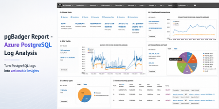
Sometimes the fastest way to understand a PostgreSQL workload is not another dashboard. It is a good log report. pgBadger is a PostgreSQL log analysis tool that turns raw PostgreSQL logs into an interactive HTML report. It helps summarize query activity, connection patterns, errors, temporary files, lock waits, autovacuum activity, and more. Earlier guidance for generating pgBadger reports from Azure Database for PostgreSQL Flexible Server focused on exporting logs through Diagnostic Settings, storing them in a storage account, and then using tools such as BlobFuse and jq to extract PostgreSQL log lines from JSON files. That workflow is still useful when customers centralize logs across multiple servers. However, if you are already using the Server logs feature in Azure Database for PostgreSQL Flexible Server, there is a much simpler path. In this post: You’ll learn how to generate a pgBadger HTML report from Azure Database for PostgreSQL Flexible Server by downloading native PostgreSQL .log files directly from the Azure portal. No storage account, BlobFuse mount, or JSON extraction required. Fast path Configure log_line_prefix . Enable Server logs for download. Download the PostgreSQL .log files. Run pgBadger with the matching prefix. Open pgbadger-report.html . Why use this workflow? With Server logs, you can download native PostgreSQL .log files directly from the Azure portal and run pgBadger locally. Older path Simpler path in this blog Diagnostic Settings → Storage account → BlobFuse → JSON extraction → pgBadger Server logs → Download .log files → pgBadger Area Older Diagnostic Settings workflow Server logs workflow Export path Diagnostic Settings to storage account Download .log files directly from the portal Format JSON payloads need extraction Native PostgreSQL .log files Extra tooling BlobFuse and jq JSON parsing None Best suited for Centralized or multi-server logging Quick per-server analysis Outcome Flexible, but more setup Faster path to pgBadger Recommended: Use the Server logs workflow when you want a fast, low-friction way to generate a pgBadger report from one Azure Database for PostgreSQL Flexible Server. When should you use this workflow? Use this workflow when... Use Diagnostic Settings when... You need a quick report for one Flexible Server. You centralize logs from many servers. You want to run pgBadger locally. You need long-term retention or workspace-level querying. You want to avoid JSON extraction. You already have automated log export pipelines. Before you start A machine where you can install or run pgBadger. A working Perl runtime. Git Bash on Windows, so the multi-line shell commands work as shown. Portal access to your Azure Database for PostgreSQL Flexible Server. Permission to update server parameters and enable Server logs. Important: pgBadger can only analyze what PostgreSQL logs capture. To populate query timing and slow-query sections in the report, enable log_min_duration_statement before collecting logs. Logs collected before that change will not include duration data. Workflow overview Task Type Rough effort Install or prepare pgBadger One-time setup per analysis machine 5–10 minutes Configure log_line_prefix One-time setup per server 2–3 minutes Enable Server logs One-time setup per server 2–3 minutes Download logs and run pgBadger Repeatable 2–5 minutes Install or prepare pgBadger on the machine where you will analyze logs. Configure log_line_prefix so pgBadger can parse each log line. Enable Server logs, so PostgreSQL logs are available for download. Download the logs and run pgBadger locally. 💡Pro tip: Start with a narrow log window first. Use one or two hourly log files, confirm the report looks right, and then expand the analysis window if needed. Step 1: Install pgBadger Before generating a report, you need pgBadger available on the machine where you plan to analyze the downloaded PostgreSQL log files. Run this on a Linux VM, WSL, or another Linux-based environment where you can install packages. Note: Azure Cloud Shell may work for quick testing, but package installation and build-tool availability can vary by session. For repeatable analysis, use a Linux VM, WSL, or another environment you control. Copy and run sudo apt-get update && sudo apt-get install -y git perl make gcc && \ git clone https://github.com/darold/pgbadger.git && \ cd pgbadger && \ perl Makefile.PL && \ make && \ sudo make install && \ pgbadger -V What good looks like: The install command completes successfully and pgbadger -V returns the installed pgBadger version. Step 2: Configure log_line_prefix This is a one-time server configuration step. The log_line_prefix parameter controls the beginning of each PostgreSQL log line. pgBadger uses this prefix to extract useful fields such as timestamp, user, database, and process ID. In the Azure portal, open your Flexible Server and go to Server parameters. Search for: Parameter log_line_prefix Set this value %m user=%u db=%d pid=%p: Then select Save. In Server parameters, confirm that the custom value is saved for log_line_prefix . Figure 1: Set log_line_prefix so pgBadger can correctly parse timestamp, user, database, and process ID from each log line. Prefix tokens Token Meaning %m Timestamp with milliseconds %u Username %d Database name %p Process ID After this change, log lines should look like this: Example log line 2026-06-22 19:00:00.070 UTC user=pgadmin db=highcpu pid=3805603: LOG: statement: SELECT 1 FROM pg_extension WHERE extname='pg_stat_statements' The matching pgBadger prefix for this log format is: Matching pgBadger prefix %m user=%u db=%d pid=%p: You will use this same value later in the pgBadger command. What good looks like: The server parameter is saved, and new PostgreSQL log lines begin with timestamp, user, database, and process ID fields that match the pgBadger prefix. Step 3: Enable Server logs for download This is also a one-time setup step. In the Azure portal, open your Flexible Server and go to Server logs. Enable: Portal setting Capture logs for download Set the retention period based on how long you want logs to remain available for download. For example, a 7-day retention period keeps logs available for download for 7 days. In Server logs, enable Capture logs for download and choose the retention window. Figure 2: Enable Capture logs for download and set a retention period long enough to cover the analysis window you want to inspect. What good looks like: After Server logs are enabled, hourly PostgreSQL log files appear in the Server logs blade and can be downloaded from the Azure portal. Once enabled, hourly log files appear in the Server logs blade. The files are named by date and hour, for example: Example log files postgresql_2026_06_22_19_00_00.log postgresql_2026_06_22_20_00_00.log Step 4: Download and organize the logs locally From the Server logs page, select the .log files for the time window you want to analyze and download them. For example, to analyze activity between 19:00 and 21:00 UTC, download: Example files to download postgresql_2026_06_22_19_00_00.log postgresql_2026_06_22_20_00_00.log On your local machine, create a folder for that analysis window. A simple convention is to use the Mon-DD format. Folder name Jun-22 Place the downloaded .log files inside that folder. Your local folder structure should look like this: Folder structure pgbadger-13.1/ pgbadger Jun-22/ postgresql_2026_06_22_19_00_00.log postgresql_2026_06_22_20_00_00.log Step 5: Generate the pgBadger report Open Git Bash from the folder where pgBadger is located. For example, if pgBadger is inside the pgbadger-13.1 folder, open Git Bash from that folder. # Action Command 1 Set the folder FOLDER=Jun-22 2 Confirm files ls -lh ./$FOLDER 3 Run pgBadger Use the full command below. Copy and run FOLDER=Jun-22 ls -lh ./$FOLDER perl -X ./pgbadger -f stderr \ --prefix '%m user=%u db=%d pid=%p:' \ ./$FOLDER/*.log \ -o ./$FOLDER/pgbadger-report.html Command breakdown Part of command Purpose perl -X ./pgbadger Runs pgBadger and suppresses non-critical Perl warnings. -f stderr Parses PostgreSQL stderr log files. --prefix '%m user=%u db=%d pid=%p:' Matches the log_line_prefix set on the server. ./$FOLDER/*.log Analyzes every .log file in the selected folder. -o ./$FOLDER/pgbadger-report.html Writes the HTML report into the same folder. When the command completes successfully, you should see output like this: Expected output Parsed 12134249 bytes of 12134249 (100.00%), queries: 26684, events: 83 LOG: Ok, generating html report... What good looks like: pgBadger finishes parsing the logs and creates pgbadger-report.html in the selected folder. Step 6: Open the report Open the generated report: Copy and run start ./$FOLDER/pgbadger-report.html The report opens in your default browser. The final report is created here: Generated report path Jun-22/pgbadger-report.html What the report can show The pgBadger report gives you a quick view into the workload shape for the selected log window. For example, in a sample run across two hourly log files, pgBadger summarized: Total number of queries. Number of unique normalized queries. Query traffic over time. Events such as errors and fatal messages. Session and connection patterns. Once the report opens, start with Global Stats to confirm the time range, total queries, normalized queries, and query peak. Figure 3: Start with Global Stats to validate the selected time range, total query count, normalized query count, and query peak. Query volume and normalized queries Many raw queries can often reduce to a smaller number of normalized query patterns. This helps identify whether the workload is spread across many different query shapes or dominated by a smaller set of repeated statements. Example: In this sample run, 26,684 queries reduced to 59 normalized query shapes. That suggests the workload is mostly a small set of repeated statements, which can help focus tuning effort. Traffic patterns The SQL Traffic section helps identify spikes, quiet periods, and workload changes over time. Figure 4: Use SQL Traffic to identify query spikes, quiet periods, and workload changes during the selected log window. Figure 5: Review the query breakdown to compare read vs. write volume and query-type distribution for the selected Server logs window. For example, if the report shows a steady baseline followed by a sharp spike, that spike can be correlated with application activity, batch jobs, synthetic tests, or operational events during the same time window. Query duration If query duration shows 0 ms or the slow query sections are empty, it usually means duration logging was not enabled when the logs were collected. In that case, pgBadger can still show query counts and events, but it cannot calculate the slowest queries, total execution time, average duration, or maximum duration. To unlock those timing sections, enable log_min_duration_statement , collect fresh logs, and rerun pgBadger. What pgBadger cannot infer from missing logs pgBadger reports are only as complete as the log data you provide. If PostgreSQL did not log duration, lock waits, temporary files, or autovacuum activity during the selected time window, pgBadger cannot reconstruct those details later. To analyze... Enable before collecting logs Slow queries log_min_duration_statement Lock waits log_lock_waits Temporary files log_temp_files Autovacuum activity log_autovacuum_min_duration Repeatable copy/paste block Reusable command block Change only FOLDER for each new analysis window. Copy and run FOLDER=Jun-22 ls -lh ./$FOLDER perl -X ./pgbadger -f stderr \ --prefix '%m user=%u db=%d pid=%p:' \ ./$FOLDER/*.log \ -o ./$FOLDER/pgbadger-report.html start ./$FOLDER/pgbadger-report.html For another date, change only this line: Update this value FOLDER=Jun-22 Examples: Example folder values FOLDER=Jun-23 FOLDER=Jul-01 FOLDER=Aug-15 Optional: Improve report quality pgBadger can only analyze the information captured in PostgreSQL logs. The default logs may be enough for query frequency, connection activity, and errors. For deeper performance troubleshooting, consider enabling additional logging parameters based on your scenario. Scenario Parameter Suggested value Notes Slow query analysis log_min_duration_statement 1000 Logs statements slower than 1 second. Short controlled test log_min_duration_statement 0 Logs every statement. Use carefully. Lock troubleshooting log_lock_waits on Helps identify lock waits. Temporary file analysis log_temp_files 0 Logs all temporary files. Autovacuum visibility log_autovacuum_min_duration 0 Useful during focused analysis. Useful parameters include: Recommended logging parameters log_lock_waits = on log_temp_files = 0 log_autovacuum_min_duration = 0 To capture query durations, configure: Duration logging log_min_duration_statement = 1000 This logs statements that run longer than 1000 milliseconds. For short test runs, you can temporarily use: Short test run only log_min_duration_statement = 0 Caution: Use log_min_duration_statement = 0 carefully on busy production servers. It logs every statement and can generate a large volume of logs. Duration matters: If duration logging is not enabled, pgBadger can still show query counts and events, but slowest-query, total duration, average duration, and maximum duration sections will be limited or empty. Common mistakes and quick fixes Symptom Likely cause Fix Report is empty Prefix mismatch Match --prefix with log_line_prefix . No duration data Duration logging was not enabled Set log_min_duration_statement before collecting logs. No files visible Server logs disabled or retention expired Enable capture and check retention. pgBadger command fails pgBadger is not in the current folder or path Run pgbadger -V to confirm installation. Common troubleshooting FAQs 1. Report is created but empty This usually means the pgBadger prefix did not match the actual log format. Check the first few lines: Copy and run head -5 ./$FOLDER/*.log Make sure the pgBadger --prefix matches the server’s log_line_prefix . 2. Report shows queries but no duration PostgreSQL logged statements but did not log durations. Enable one of the following, collect fresh logs, and rerun pgBadger: Parameter options log_min_duration_statement = 1000 # or temporarily for testing log_min_duration_statement = 0 3. No .log files are visible Confirm that Server logs are enabled: Portal setting Capture logs for download Also check the retention period. If the retention period has expired, older logs may no longer be available for download. 4. pgBadger command fails Confirm that pgBadger is available in the current folder or installed in your path. Copy and run pgbadger -V If you are running pgBadger from the local folder, use: Copy and run perl -X ./pgbadger Summary For customers already using Azure Database for PostgreSQL Flexible Server logs, the pgBadger workflow is straightforward: Install pgBadger. Configure log_line_prefix . Enable Server logs for download. Download the .log files. Place them in a local date-based folder. Run pgBadger with the matching prefix. Open pgbadger-report.html . Bottom line: Server logs give you the shortest path from Azure Database for PostgreSQL Flexible Server logs to a pgBadger report. Download the native .log files, run pgBadger with the matching prefix, and open the generated HTML report. References pgBadger - source and documentation GitHub pgBadger - project site Azure - Download server logs from the portal Flexible Server Azure - Logging concepts Flexible Server Azure - Configure server parameters via the portal PostgreSQL - log_line_prefix and logging parameters660Views2likes0CommentsLessons Learned #547:Some SQL DB Statistics Remain Outdated While Others Are Automatically Updated
During the analysis of a SQL Server performance case, we observed an interesting statistics update pattern on a large table. Several statistics had recently been updated at different times, while a group of automatically created _WA_Sys_ statistics still showed: An older last_updated date. A high modification_counter. A row count significantly lower than the current number of rows in the table. At first glance, this could suggest that AUTO_UPDATE_STATISTICS was not working correctly. However, a closer review showed that this pattern can be completely consistent with the expected behavior of SQL Server. 1. Types of statistics in SQL Server SQL Server can maintain several types of statistics. Automatically created column statistics When AUTO_CREATE_STATISTICS is enabled, SQL Server can automatically create a single-column statistic when the Query Optimizer needs cardinality information for a column used in a query predicate. These statistics normally use names such as: _WA_Sys_00000002_47A6D5E5 The name can be interpreted as: _WA_Sys_<column_id in hexadecimal>_<object_id in hexadecimal> For example: 00000002 hexadecimal = column_id 2 47A6D5E5 hexadecimal = table object_id The most reliable way to identify the associated column is not to decode the name manually, but to query the SQL Server catalog views: DECLARE @TableName sysname = N'dbo.CustomerTransactions'; SELECT s.stats_id, s.name AS statistics_name, sc.stats_column_id, c.column_id, c.name AS column_name, s.auto_created, s.user_created, s.no_recompute FROM sys.stats AS s INNER JOIN sys.stats_columns AS sc ON sc.object_id = s.object_id AND sc.stats_id = s.stats_id INNER JOIN sys.columns AS c ON c.object_id = sc.object_id AND c.column_id = sc.column_id WHERE s.object_id = OBJECT_ID(@TableName) AND s.name = N'_WA_Sys_00000002_47A6D5E5' ORDER BY sc.stats_column_id; Statistics associated with indexes When SQL Server creates an index, it also creates a statistics object associated with the index. For example: CREATE INDEX IX_CustomerTransactions_ClientId ON dbo.CustomerTransactions(ClientId) this creates an index statistics object normally named: IX_CustomerTransactions_ClientId when a statistics object corresponds to an index, its stats_id matches the index's index_id. User-created statistics Statistics can also be created explicitly: CREATE STATISTICS ST_CustomerTransactions_ClientId_Status ON dbo.CustomerTransactions ( ClientId, StatusId ); This object is identified in sys.stats with: user_created = 1 auto_created = 0 and AUTO_UPDATE_STATISTICS applies to index statistics, automatically created single-column statistics, manually created statistics and filtered statistics. 2. Statistics are not updated together Assume that a table has these statistics: _WA_Sys_00000002_xxxxxxxx for ClientId _WA_Sys_00000003_xxxxxxxx for StatusId IX_CustomerTransactions_CreatedDate for CreatedDate PK_CustomerTransactions and TransactionId After a large data load, several or all of them could become eligible for an automatic update. However, SQL Server does not immediately update all eligible statistics. Before compiling a query, the Query Optimizer identifies the statistics that could be relevant to the query predicates and checks whether those statistics are outdated. Consider this query: SELECT TransactionId, ClientId, Amount FROM dbo.CustomerTransactions WHERE ClientId = 100; The optimizer might need a histogram on ClientId. If the corresponding statistics object is outdated and has crossed its update threshold, SQL Server may update that specific statistics object. It does not need to update unrelated statistics on: StatusId CreatedDate As a result, statistics on the same table can legitimately have different update times: PK_CustomerTransactions 2026-07-22 10:53 IX_CustomerTransactions_ClientId 2026-07-22 10:50 IX_CustomerTransactions_CreatedDate 2026-07-22 10:13 _WA_Sys_00000003_47A6D5E5 2026-07-19 10:00 This pattern can be evidence of demand-driven automatic updates rather than evidence of a malfunction. 3. What does modification_counter represent? The modification_counter returned by sys.dm_db_stats_properties represents the number of modifications made to the leading statistics column since that statistics object was last updated. This definition is especially important for multicolumn statistics. For example: CREATE INDEX IX_CustomerTransactions_ClientId_Status ON dbo.CustomerTransactions ( ClientId, StatusId ); The associated statistics object contains: Histogram: ClientId Density information: ClientId ClientId, StatusId The histogram and modification_counter are based on the leading column, ClientId. If only StatusId is modified: UPDATE dbo.CustomerTransactions SET StatusId = 2 WHERE TransactionId = 100; this does not have the same statistics impact as changing ClientId, because ClientId is the leading histogram column. SQL Server statistics contain only one histogram, built on the first key column. Multicolumn statistics additionally contain density information for column prefixes. 4. Why do multiple statistics sometimes have similar modification counters? This commonly happens after an insert operation. For example: INSERT INTO dbo.CustomerTransactions ( TransactionId, ClientId, StatusId, Amount, CreatedDate ) SELECT TransactionId, ClientId, StatusId, Amount, CreatedDate FROM dbo.StagingCustomerTransactions; Each inserted row introduces a value for every populated column. Consequently, multiple single-column statistics may show similar increases in their modification counters. This is particularly visible after a large ETL operation: Table rows before the load: 487,673 Rows inserted by the ETL: 515,244 Current approximate row count: 1,002,917 Several statistics could then show modification counters close to the number of inserted rows. That does not mean SQL Server must update all those statistics immediately. They become candidates for updating, but an update is normally triggered when query optimization requires them. 5. Does automatic updating apply only to _WA_Sys_ statistics? AUTO_UPDATE_STATISTICS applies to: Automatically created _WA_Sys statistics Index statistics Primary-key index statistics User-created statistics Each statistics object is evaluated independently. Therefore, SQL Server might update: PK_CustomerTransactions while leaving this object unchanged: _WA_Sys_00000003_47A6D5E5 The reverse is also possible. The behavior depends on which statistics are considered relevant during compilation or cached-plan validation. 6. What happens when a _WA_Sys_ statistic and an index statistic cover the same column? This is one of the most interesting scenarios. Assume SQL Server originally created: _WA_Sys_00000002_xxxxxxxx for ClientId. Later, someone creates this index: CREATE INDEX IX_CustomerTransactions_ClientId ON dbo.CustomerTransactions(ClientId); The table now has two statistics objects with histograms on ClientId: _WA_Sys_00000002_xxxxxxxx and IX_CustomerTransactions_ClientId Conceptually: _WA_Sys statistic Histogram on ClientId Index statistic Histogram on ClientId For a query such as: SELECT * FROM dbo.CustomerTransactions WHERE ClientId = @ClientId; the optimizer can have more than one potentially relevant statistics object. It may rely on the index statistics object rather than the older _WA_Sys_ object. In that case: IX_CustomerTransactions_ClientId Updated recently _WA_Sys_00000002_xxxxxxxx Old last_updated value High modification_counter This does not necessarily mean that automatic statistics updating has failed. It can mean that the _WA_Sys_ statistic has become redundant and has not been required by recent compilations. However, this should be presented carefully: The Query Optimizer is not publicly documented as always preferring an index statistic over an equivalent _WA_Sys_ statistic. The statistics selected can depend on: Query. Predicates. Available indexes. Filtered versus unfiltered statistics. Statistics freshness. Sampling quality. Multicolumn density information. Cardinality Estimator behavior. Existing cached plans. The correct conclusion is that the scenario is possible and plausible, but the execution plan should be inspected before claiming that a specific statistics object was used. As we wrote down in multiple articles in our blog (below), identify redudant statistics is part of DBA work to avoid this situation, also, in other situations, I saw that the maintenance plan is taking too much time because we are updating statistics that we are not using or migth be duplicated. The following script identifies statistics whose leading columns overlap: DECLARE @TableName sysname = N'dbo.CustomerTransactions'; ;WITH LeadingStatisticsColumns AS ( SELECT s.object_id, s.stats_id, s.name AS statistics_name, s.auto_created, s.user_created, s.no_recompute, s.has_filter, s.filter_definition, sc.column_id, c.name AS leading_column, i.index_id, i.name AS index_name FROM sys.stats AS s INNER JOIN sys.stats_columns AS sc ON sc.object_id = s.object_id AND sc.stats_id = s.stats_id AND sc.stats_column_id = 1 INNER JOIN sys.columns AS c ON c.object_id = sc.object_id AND c.column_id = sc.column_id LEFT JOIN sys.indexes AS i ON i.object_id = s.object_id AND i.index_id = s.stats_id WHERE s.object_id = OBJECT_ID(@TableName) ) SELECT leading_column, statistics_name, CASE WHEN index_id IS NOT NULL THEN N'INDEX STATISTICS' WHEN auto_created = 1 THEN N'AUTO-CREATED _WA_SYS' WHEN user_created = 1 THEN N'USER-CREATED STATISTICS' ELSE N'OTHER' END AS statistics_type, index_name, has_filter, filter_definition, no_recompute, COUNT(*) OVER ( PARTITION BY column_id ) AS statistics_on_same_leading_column FROM LeadingStatisticsColumns ORDER BY leading_column, statistics_type, statistics_name; This does not automatically mean that one object should be deleted. It only identifies an overlap. 7. Script The following example demonstrates how an automatically created statistic can coexist with a later index statistic. DROP TABLE IF EXISTS dbo.CustomerTransactions; GO CREATE TABLE dbo.CustomerTransactions ( TransactionId int NOT NULL, ClientId int NOT NULL, StatusId tinyint NOT NULL, Amount decimal(12,2) NOT NULL, CreatedDate datetime2(0) NOT NULL, CONSTRAINT PK_CustomerTransactions PRIMARY KEY CLUSTERED (TransactionId) ); GO Insert sample data ;WITH Numbers AS ( SELECT TOP (200000) ROW_NUMBER() OVER ( ORDER BY (SELECT NULL) ) AS n FROM sys.all_objects AS a CROSS JOIN sys.all_objects AS b ) INSERT INTO dbo.CustomerTransactions ( TransactionId, ClientId, StatusId, Amount, CreatedDate ) SELECT n, n % 5000, n % 5, CONVERT(decimal(12,2), n % 10000), DATEADD ( minute, -(n % 100000), SYSUTCDATETIME() ) FROM Numbers; GO Ensure that automatic statistics creation and updating are enable ALTER DATABASE CURRENT SET AUTO_CREATE_STATISTICS ON; GO ALTER DATABASE CURRENT SET AUTO_UPDATE_STATISTICS ON; GO Trigger automatic statistics creation on ClientId SELECT COUNT_BIG(*) FROM dbo.CustomerTransactions WHERE ClientId = 100 OPTION (RECOMPILE); GO Check the statistics created for ClientId SELECT s.stats_id, s.name AS statistics_name, s.auto_created, s.user_created, c.name AS column_name FROM sys.stats AS s INNER JOIN sys.stats_columns AS sc ON sc.object_id = s.object_id AND sc.stats_id = s.stats_id INNER JOIN sys.columns AS c ON c.object_id = sc.object_id AND c.column_id = sc.column_id WHERE s.object_id = OBJECT_ID(N'dbo.CustomerTransactions') AND c.name = N'ClientId' ORDER BY s.stats_id; Create an index on the same column CREATE INDEX IX_CustomerTransactions_ClientId ON dbo.CustomerTransactions(ClientId); The table can now have: Modify the data significantly UPDATE dbo.CustomerTransactions SET ClientId = ClientId + 10000 WHERE TransactionId <= 100000; Review the counters again SELECT s.name AS statistics_name, sp.last_updated, sp.rows, sp.rows_sampled, sp.modification_counter FROM sys.stats AS s OUTER APPLY sys.dm_db_stats_properties ( s.object_id, s.stats_id ) AS sp WHERE s.object_id = OBJECT_ID(N'dbo.CustomerTransactions') ORDER BY s.stats_id Force a new compilation using ClientId SET STATISTICS XML ON; GO SELECT COUNT_BIG(*) FROM dbo.CustomerTransactions WHERE ClientId = 10100 OPTION (RECOMPILE); GO SET STATISTICS XML OFF; GO After the query, review: The actual execution plan XML. The StatisticsInfo elements. last_updated. modification_counter. The exact object updated is an optimizer decision and can vary by SQL Server version, build, compatibility level and query shape. The test should therefore be used to observe the behavior rather than to assume a fixed preference. Finally, as you could see SQL Server choose _WA_Sys_00000002_151102AD instead of IX_CustomerTransactions_ClientId to update. In some situations, depending on execution plan, SQL Server might choose IX_CustomerTransactions_ClientId to update instead of _WA_Sys_00000002_151102AD and for this reason, doesn't mean that SQL Server is not updating the statistics it is depending that it is choosing one of them that the column is involved. My lessons learned, a statistic can be outdated without being relevant, and it can be relevant without being the only available source of cardinality information. Before interpreting an old last_updated value as an automatic statistics failure, identify the leading column, look for overlapping statistics, inspect the execution plan and determine whether there is a real estimation or performance problem. Articles: Lesson Learned #482: Identifying Potential Duplicate Statistics | Microsoft Community Hub Lesson Learned #324: Query Recompilation in Azure SQL | Microsoft Community Hub Lessons Learned #537: Copilot Prompts for Troubleshooting on Azure SQL Database | Microsoft Community Hub Lesson Learned #498:Understanding the Role of STATMAN in SQL Server and Its Resource Consumption | Microsoft Community Hub Disclaimer: The scripts included in this article are provided for demonstration and educational purposes only. They create a sample table, insert a significant number of rows, create indexes and statistics, modify data, and change automatic statistics settings in the current database. Run the complete demonstration only in a test or non-production environment. Review and adapt the database name, object names, row volume, and statements before execution. The results may vary depending on the SQL Server version, database compatibility level, existing configuration, data distribution, and workload. Always test the scripts in a representative environment before applying any conclusion or change to a production system.292Views0likes0CommentsLessons Learned #544: How to Detect INT Identity Exhaustion Before Inserts Fail.
Recently, I worked on a support case involving an Azure SQL Database table where the customer had reached the maximum value supported by the INT data type. The table used an INT IDENTITY(1,1) column as its primary key. Over time, the generated identity value approached the maximum value supported by INT. Once the available range was exhausted, the application was no longer able to insert new rows. At that point, the column needed to be changed from INT to BIGINT. However, performing this type of migration on a very large table can be a complex and time-consuming operation. The situation is that an INT column uses 4 bytes and supports values from: -2,147,483,648 to: 2,147,483,647. To prevent similar problems in the future, I suggested using the following query to review the current status of all INT IDENTITY columns in the database. The query uses the sys.identity_columns catalog view: SELECT s.name AS SchemaName, t.name AS TableName, c.name AS ColumnName, CONVERT(bigint, c.last_value) AS CurrentIdentityValue, CONVERT(bigint, 2147483647) AS MaximumIntValue, CONVERT(bigint, 2147483647) - ISNULL(CONVERT(bigint, c.last_value), 0) AS RemainingValues, CAST( ISNULL(CONVERT(decimal(20,2), c.last_value), 0) / 2147483647 * 100 AS decimal(6,2) ) AS PercentUsed FROM sys.identity_columns AS c INNER JOIN sys.tables AS t ON c.object_id = t.object_id INNER JOIN sys.schemas AS s ON t.schema_id = s.schema_id WHERE TYPE_NAME(c.system_type_id) = 'int' ORDER BY PercentUsed DESC; I prefer using this query instead of relying on: SELECT COUNT(*) FROM dbo.TableName. The number of rows in a table does not necessarily match the current identity value. Rows might have been deleted, transactions might have been rolled back, and identity values might contain gaps. For this reason, the current identity value is a better indicator of the remaining capacity. Adding this query as a regular preventive check can help identify identity columns that are approaching their limits before they cause application failures. I would like to share with you an example creates a table with an identity seed close to the maximum value supported by INT: DROP TABLE IF EXISTS dbo.IdentityCapacityDemo2; CREATE TABLE dbo.IdentityCapacityDemo2 ( Id INT IDENTITY(2147483600,1) NOT NULL, CreatedDate datetime2(0) NOT NULL CONSTRAINT DF_IdentityCapacityDemo2_CreatedDate DEFAULT SYSUTCDATETIME(), CONSTRAINT PK_IdentityCapacityDemo2 PRIMARY KEY CLUSTERED (Id) ) Insert 20 rows using this command: insert into IdentityCapacityDemo2(CreatedDate) values(SYSUTCDATETIME()) Example of returns: I think runnning this preventive check can help detect identity exhaustion before it affects the application.