hpc
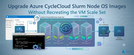
278 TopicsUpgrade Azure CycleCloud Slurm Node OS Images Without Recreating the VM Scale Set
Overview Operating-system image updates in an Azure CycleCloud Slurm cluster are not the same as installing ordinary packages inside a running node. A CycleCloud Slurm node is typically an instance in an Azure Virtual Machine Scale Set (VMSS), and the VMSS model defines the image from which its OS disk is created. This distinction is especially important when the VMSS uses Manual upgrade mode. Changing an image setting does not automatically upgrade running instances. Likewise, reimaging a node without first changing the VMSS model can rebuild that node from the same old image. This article describes a controlled, node-by-node method for moving an existing CycleCloud-managed Slurm partition from one Ubuntu HPC image version to another without deleting and recreating the entire VMSS. NOTE: The same procedure can be used for other schedulers. The appropriate scheduler specific commands need to used for node servicing. The validated example changes the image reference from: microsoft-dsvm:ubuntu-hpc:2404:24.04.2026052601 to: microsoft-dsvm:ubuntu-hpc:2404:24.04.2026092501 These versions are examples from the validated procedure. Always select and validate an image appropriate for your region, VM size, kernel, drivers, scheduler integration, and application stack. Problem statement A CycleCloud Slurm cluster may have long-running compute or GPU nodes that require a newer OS image for reasons such as: Security and compliance updates Kernel fixes Updated device drivers Platform fixes Updated HPC libraries Standardization on a newer image baseline Application or container-runtime compatibility Supportability requirements The most straightforward lifecycle operation is often to update the image in CycleCloud, scale the partition down, allow CycleCloud to remove the old VMSS, and then scale the partition back up. CycleCloud then creates a new VMSS using the updated image. Although that method provides a clean deployment, it may be undesirable in a busy HPC environment because: The complete partition may need a maintenance window. All nodes in the partition may become unavailable together. Deleting the scale set deliberately releases the partition’s current VM allocations. Capacity must be acquired again when the partition is restarted. Azure capacity is dynamic and cannot always be guaranteed at the time of reacquisition. Validation happens after a larger infrastructure change instead of on a single canary node. A deployment problem can affect the entire partition rather than one selected instance. Large distributed workloads may take significant time to drain from the full partition. Administrators may therefore need a method that updates the OS image of selected idle nodes while the remaining nodes continue serving workloads. The challenge is that three separate states must be understood and managed: CycleCloud cluster configuration The image definition CycleCloud will use when it creates or recreates infrastructure. VMSS model The image reference currently defined on the existing scale set. VMSS instance state Whether a particular VMSS instance has applied the latest VMSS model. If these three states are not handled in the correct order, a reimage can complete successfully while leaving the node on the old image. Why reimage alone does not solve the problem A reimage replaces the node’s OS disk using the image and configuration associated with its current infrastructure model. Reimage does not, by itself, select a newer OS image. This creates a common failure pattern: The desired image is changed in the CycleCloud cluster configuration. The existing VMSS continues to reference the old image. A CycleCloud, Slurm, or VMSS reimage action is initiated. The OS disk is rebuilt. The node returns using the old image because the VMSS model still references that image. For a VMSS configured with Manual upgrade mode, the required order is: Drain the selected Slurm node. Change the image reference in the existing VMSS model. Confirm the new image in the VMSS model. Confirm that existing instances report LatestModelApplied=False. Apply the latest model to one selected instance using az vmss update-instances. Wait for the node to return. Confirm that the selected instance reports LatestModelApplied=True. Verify the new image from inside the VM. Validate the OS, scheduler, drivers, network fabric, container runtime, and workload. Resume the node. Repeat for the remaining instances. Update the CycleCloud node-array image configuration to prevent configuration drift. Advantages of this approach No full VMSS recreation The existing VMSS object is updated in place. The process does not intentionally delete the complete scale set and create a replacement. Node-level maintenance Only the selected VMSS instance is disrupted. Other nodes can remain available, provided that the workload and cluster architecture support node-by-node maintenance. Canary validation One idle node can be upgraded first. The new image can be tested against the actual scheduler, drivers, network, containers, and applications before expanding the change. Smaller failure domain If the first upgraded node fails validation, it can remain drained while the remaining nodes continue using the previous image. Reduced capacity exposure The procedure avoids deliberately scaling the entire partition to zero and releasing all current allocations at once. This can reduce exposure to capacity reacquisition risk. However, it should not be treated as a guarantee that host placement or capacity will never change during platform servicing. Controlled scheduling Nodes can be upgraded as they become idle. Slurm drain and resume operations create a clear boundary between: Workload evacuation Infrastructure servicing Technical validation Return to production Measurable rollout progress The latestModelApplied property provides an explicit signal showing which VMSS instances have received the updated model. Easier rollback control If the canary node fails, the rollout can stop before all nodes are changed. This is generally easier to manage than recovering an entire recreated partition. Important limitations This is a rolling infrastructure procedure, not a zero-downtime operation. The selected node becomes unavailable while its OS disk is serviced. Jobs running on that node must complete, migrate, be requeued, or be stopped. Multi-node MPI and distributed training jobs may make node-by-node maintenance impractical. A partition-wide maintenance window may be safer when jobs span most or all nodes. Data or configuration stored only on the OS disk may be lost during servicing. Node bootstrap should be reproducible and important state should be stored externally. Containers do not isolate applications from every host change. The host kernel, GPU driver, RDMA stack, device plugins, mounts, and scheduler integration remain important to containerized workloads. A direct VMSS update does not permanently update the CycleCloud cluster definition. CycleCloud must be updated after successful validation to prevent configuration drift. Prerequisites Before starting, confirm the following: The target node belongs to the expected CycleCloud-managed VMSS. The VMSS uses Manual upgrade mode. The target image has been selected and validated for the environment. The target image is available for the required region and VM size. You have Azure permissions to read and update the VMSS and its instances. (Contributor or Virtual Machine contributor role for the subscription) Azure CLI is installed and authenticated in the correct tenant and context. jq is available on the Linux node for metadata formatting. You have Slurm administrative permission to drain and resume nodes. Required application and configuration state is not stored only on the OS disk. A maintenance window has been approved. A rollback plan has been documented. The first target is an idle or noncritical canary node. Define placeholders instead of embedding environment-specific values: RESOURCE_GROUP="<RESOURCE-GROUP>" VMSS_NAME="<VMSS-NAME>" INSTANCE_ID="<INSTANCE-ID>" SLURM_NODE="<SLURM-NODE-NAME>" TARGET_IMAGE_VERSION="24.04.2026092501" PREVIOUS_IMAGE_VERSION="24.04.2026052601" Detailed upgrade procedure Step 1: Capture the current image from inside the HPC compute node Run the following on the target VM. curl -s -H Metadata:true --noproxy "" "http://169.254.169.254/metadata/instance/compute?api-version=2021-10-01" | jq '{publisher, offer, sku, version, osType}' Output: { "publisher": "microsoft-dsvm", "offer": "ubuntu-hpc", "sku": "2404", "version": "24.04.2026052601", "osType": "Linux" } Also record the current OS release and kernel: cat /etc/os-release uname -r Keep these results in the change record. They provide the baseline needed to prove that the image changed after the operation. vinil@”$SLURM_NODE”:~$ cat /etc/os-release PRETTY_NAME="Ubuntu 24.04.4 LTS" NAME="Ubuntu" VERSION_ID="24.04" VERSION="24.04.4 LTS (Noble Numbat)" VERSION_CODENAME=noble ID=ubuntu ID_LIKE=debian HOME_URL="https://www.ubuntu.com/" SUPPORT_URL="https://help.ubuntu.com/" BUG_REPORT_URL="https://bugs.launchpad.net/ubuntu/" PRIVACY_POLICY_URL="https://www.ubuntu.com/legal/terms-and-policies/privacy-policy" UBUNTU_CODENAME=noble LOGO=ubuntu-logo vinil@”$SLURM_NODE”:~$ uname -r 6.8.0-1054-azure Step 2: Confirm the VMSS upgrade mode and current image Run the following from Azure Cloud Shell: az vmss show --resource-group "$RESOURCE_GROUP" --name "$VMSS_NAME" --query "{UpgradeMode:upgradePolicy.mode,Image:virtualMachineProfile.storageProfile.imageReference}" --output json Sanitized output: { "Image": { "offer": "ubuntu-hpc", "publisher": "microsoft-dsvm", "sku": "2404", "version": "24.04.2026052601" }, "UpgradeMode": "Manual" } The important value is: "UpgradeMode": "Manual" With Manual upgrade mode, changing the VMSS model does not automatically update existing instances. Do not continue until the current image and upgrade mode match the change plan. Step 3: Map Slurm nodes to VMSS instance IDs List all instances in the scale set: az vmss list-instances --resource-group "$RESOURCE_GROUP" --name "$VMSS_NAME" --query "[].{InstanceId:instanceId,ComputerName:osProfile.computerName,ProvisioningState:provisioningState}" --output table Output: InstanceId ComputerName ProvisioningState ------------ -------------- ------------------- 0 <NODE-000> Succeeded 1 <NODE-001> Succeeded Confirm the mapping carefully. A VMSS instance ID is not necessarily the same as a Slurm node name. For the first validation: INSTANCE_ID="0" SLURM_NODE="slurm-hpc-1" Only one instance should be selected for the canary upgrade. Step 4: Drain the selected Slurm node Prevent Slurm from scheduling new jobs on the node: SLURM_NODE="slurm-hpc-1" scontrol update NodeName="$SLURM_NODE" State=DRAIN Reason="VMSS OS image upgrade" Confirm the state: sinfo -N -n "$SLURM_NODE" Output: NODELIST NODES PARTITION STATE slurm-hpc-1 1 hpc* drain Check whether jobs are still assigned to the node: root@slurm01-scheduler:~# squeue -w "$SLURM_NODE" JOBID PARTITION NAME USER ST TIME NODES NODELIST(REASON) root@slurm01-scheduler:~# Proceed only when: The node is DRAINING while existing work completes, or DRAINED when no work remains. squeue -w returns no active jobs for the node. Dependencies involving distributed jobs have been considered. The node does not hold application state required by active workloads. Do not continue while the node is still running a workload. Step 5: Update the OS image in the VMSS model Update only the image version in the existing scale-set model: az vmss update --resource-group "$RESOURCE_GROUP" --name "$VMSS_NAME" --set virtualMachineProfile.storageProfile.imageReference.version="$TARGET_IMAGE_VERSION" The command may return a large JSON object. The important sections should contain: { "upgradePolicy": { "mode": "Manual" }, "virtualMachineProfile": { "storageProfile": { "imageReference": { "offer": "ubuntu-hpc", "publisher": "microsoft-dsvm", "sku": "2404", "version": "24.04.2026092501" } } } } At this point: The VMSS model references the target image. Existing VMSS instances have not yet been upgraded. No node should be assumed to be using the target image yet. This separation is one of the most important concepts in the procedure. Step 6: Verify the target image in the VMSS model Query only the image reference: az vmss show --resource-group "$RESOURCE_GROUP" --name "$VMSS_NAME" --query "virtualMachineProfile.storageProfile.imageReference" --output json Output: { "offer": "ubuntu-hpc", "publisher": "microsoft-dsvm", "sku": "2404", "version": "24.04.2026092501" } Do not continue until the VMSS model shows the intended target image. Step 7: Confirm that existing instances have not applied the new model Run: az vmss list-instances --resource-group "$RESOURCE_GROUP" --name "$VMSS_NAME" --expand instanceView --query "[].{InstanceId:instanceId,ComputerName:osProfile.computerName,LatestModelApplied:latestModelApplied,ProvisioningState:provisioningState}" --output table Output: InstanceId ComputerName LatestModelApplied ProvisioningState ------------ -------------- -------------------- ----------------- 0 <NODE-000> False Succeeded 1 <NODE-001> False Succeeded The important value is: LatestModelApplied=False This confirms that: The VMSS model contains the new image. The existing VMSS instances are still using their previous model. The model change has not automatically upgraded the nodes. Step 8: Apply the latest model to the canary instance Apply the updated VMSS model to only the selected instance: az vmss update-instances --resource-group "$RESOURCE_GROUP" --name "$VMSS_NAME" --instance-ids "$INSTANCE_ID" This operation is disruptive to the selected node. Its OS disk is serviced and connectivity is temporarily unavailable. Do not start another node upgrade until this instance has: Returned to a successful provisioning state. Booted correctly. Completed CycleCloud initialization. Reconnected to Slurm. Passed the complete validation checklist. Step 9: Confirm that the canary applied the latest model Run the instance-view query again: az vmss list-instances --resource-group "$RESOURCE_GROUP" --name "$VMSS_NAME" --expand instanceView --query "[].{InstanceId:instanceId,ComputerName:osProfile.computerName,LatestModelApplied:latestModelApplied,ProvisioningState:provisioningState}" --output table Expected result after upgrading instance 0: InstanceId ComputerName LatestModelApplied ProvisioningState ------------ -------------- -------------------- ----------------- 0 <NODE-000> True Succeeded 1 <NODE-001> False Succeeded This is the desired canary state: Instance 0 has applied the latest model. Instance 1 remains on the previous model. The VMSS continues to exist. The rollout can pause for detailed validation. Do not rely only on ProvisioningState=Succeeded. Confirm both the model status and the in-guest OS image. Step 10: Verify the image from inside the upgraded node After the VM becomes accessible, query its metadata again: curl -s -H Metadata:true --noproxy "" "http://169.254.169.254/metadata/instance/compute?api-version=2021-10-01" | jq '{publisher, offer, sku, version, osType}' Output { "publisher": "microsoft-dsvm", "offer": "ubuntu-hpc", "sku": "2404", "version": "24.04.2026092501", "osType": "Linux" } This confirms that the image changed from: microsoft-dsvm:ubuntu-hpc:2404:24.04.2026052601 to: microsoft-dsvm:ubuntu-hpc:2404:24.04.2026092501 Step 11: Verify the operating-system release Run: # cat /etc/os-release PRETTY_NAME="Ubuntu 24.04.5 LTS" NAME="Ubuntu" VERSION_ID="24.04" VERSION="24.04.5 LTS (Noble Numbat)" VERSION_CODENAME=noble ID=ubuntu ID_LIKE=debian HOME_URL="https://www.ubuntu.com/" SUPPORT_URL="https://help.ubuntu.com/" BUG_REPORT_URL="https://bugs.launchpad.net/ubuntu/" PRIVACY_POLICY_URL="https://www.ubuntu.com/legal/terms-and-policies/privacy-policy" UBUNTU_CODENAME=noble LOGO=ubuntu-logo Verify the running kernel: # uname -r 6.8.0-1067-azure The result should match the kernel expected for the approved target image and its driver stack. The actual kernel output should be recorded internally rather than copied into a public article if it contains environment-specific information. Step 12: Validate operating-system health # Check for failed services: systemctl --failed --no-pager # Check the overall system state: systemctl is-system-running # Review boot errors: journalctl -b -p err --no-pager # If cloud-init is used: cloud-init status --long Validation criteria should include: The node booted successfully. No unexpected failed services remain. Cloud-init or equivalent bootstrap completed. CycleCloud initialization completed. Required filesystems and application paths are available. DNS resolution works. Time synchronization is healthy. Identity and authentication components work. Monitoring and security agents are operational. No unexpected kernel or device initialization errors are present. Step 13: Validate CycleCloud and Slurm integration Confirm that Slurm can see the node: scontrol show node "$SLURM_NODE" Review the node’s: State Features Partitions CPU count Memory Generic resources Reason field Registration status The OS image upgrade may change bootstrap timing or host configuration. Confirm that CycleCloud applied the expected node configuration and that Slurm did not register the node with unexpected hardware or resource values. Step 14: Validate HPC and accelerator dependencies An OS image update can change the kernel, device drivers, user-space libraries, and bootstrap behavior. Validate every host-level dependency used by the partition. GPU validation For GPU nodes: nvidia-smi Confirm: All expected GPUs are visible. The driver initializes successfully. No unexpected device or driver errors are reported. The driver is compatible with the application and container stack. InfiniBand and RDMA validation For InfiniBand or RDMA nodes: ibv_devices ibstat Confirm: Expected devices are present. Ports are active. Link state is correct. The expected transport stack is available. Container validation For containerized environments, validate: Container runtime startup GPU device exposure RDMA device exposure Host-library injection Required mounts User namespace behavior Scheduler integration Application-specific plugins A container does not remove dependency on the host kernel, GPU driver, network device stack, or scheduler configuration. Workload validation Run representative tests such as: A single-node CPU job A GPU visibility and compute test An RDMA connectivity test An MPI or UCX smoke test A container launch test A small version of a production workload Do not treat a successful VM boot as sufficient proof that the node is production-ready. Step 15: Resume the validated node After all checks pass: scontrol update NodeName="$SLURM_NODE" State=RESUME Verify the state: sinfo -N -n "$SLURM_NODE" Confirm that: Slurm returns the node to the expected state. No unexpected drain reason remains. A small test job runs successfully. The node behaves as expected under scheduling. Step 16: Upgrade the next instance After the canary node has passed validation, select the next idle instance: INSTANCE_ID="1" SLURM_NODE="<NODE-001>" Drain it: scontrol update NodeName="$SLURM_NODE" State=DRAIN Reason="VMSS OS image upgrade" Confirm there are no jobs: sinfo -N -n "$SLURM_NODE" squeue -w "$SLURM_NODE" Apply the already-updated VMSS model: az vmss update-instances --resource-group "$RESOURCE_GROUP" --name "$VMSS_NAME" --instance-ids "$INSTANCE_ID" After the operation completes, repeat all control-plane, operating-system, scheduler, driver, network, container, and workload validation. When both example instances have been upgraded, the expected state is: InstanceId ComputerName LatestModelApplied ProvisioningState ------------ -------------- -------------------- ----------------- 0 <NODE-000> True Succeeded 1 <NODE-001> True Succeeded Repeat the drain, update, validate, and resume cycle until every intended instance reports LatestModelApplied=True and passes workload validation. Update-instances versus reimage These operations address different layers of the upgrade. Operation What it changes Key point az vmss update VMSS model Existing instances remain unchanged in Manual mode. az vmss update-instances Selected VMSS instances Applies the latest VMSS model to the selected instances. az vmss reimage Selected instance OS disks Rebuilds the OS disk but should not be treated as a substitute for applying the latest model in this workflow. CycleCloud or Slurm reimage action Requests node reimage through the cluster workflow Does not itself change an old VMSS image reference to a new one. Scale down and scale up after changing CycleCloud Recreates infrastructure from the CycleCloud definition Provides a clean deployment but may require partition-wide downtime and capacity reacquisition. The most important rule is: A reimage can reproduce the old OS if the infrastructure model still references the old image. The validated sequence is therefore: Update VMSS model verify model confirm LatestModelApplied=False run update-instances confirm LatestModelApplied=True verify the image from inside the node Prevent configuration drift in CycleCloud Directly modifying the existing VMSS is not the final configuration-management step. CycleCloud remains the owner of the cluster definition. If CycleCloud later removes and recreates the VMSS, the replacement scale set will use the image configured in the CycleCloud node array. If the CycleCloud definition still points to the previous image, newly created nodes may return to that version even though the current VMSS was upgraded manually. After the canary and rollout succeed: Update the OS image in the corresponding CycleCloud node-array configuration. Use the same publisher, offer, SKU, and version validated in the VMSS. Review or export the cluster configuration to confirm the new value is persistent. Test a controlled scale-out or node replacement if the maintenance plan permits. Record the CycleCloud configuration change with the VMSS change. The desired end state is: CycleCloud node-array image = VMSS model image = Image reported by every upgraded VMSS instance Updating only the current VMSS should not be treated as a permanent CycleCloud configuration change. Rollback strategy A rollback plan should be prepared before the first node is changed. If the canary fails validation: Keep the node drained. Stop the rollout to all remaining nodes. Capture boot, extension, driver, scheduler, and application logs. Change the VMSS model back to the previous image. Apply the previous model to the affected instance. Revalidate the restored node. Resume it only after the previous service level has been restored. Example rollback: az vmss update --resource-group "$RESOURCE_GROUP" --name "$VMSS_NAME" --set virtualMachineProfile.storageProfile.imageReference.version="$PREVIOUS_IMAGE_VERSION" Apply the restored model: az vmss update-instances --resource-group "$RESOURCE_GROUP" --name "$VMSS_NAME" --instance-ids "$INSTANCE_ID" Verify the model: az vmss show --resource-group "$RESOURCE_GROUP" --name "$VMSS_NAME" --query "virtualMachineProfile.storageProfile.imageReference" --output json Verify the instance status: az vmss list-instances --resource-group "$RESOURCE_GROUP" --name "$VMSS_NAME" --expand instanceView --query [].{InstanceId:instanceId,LatestModelApplied:latestModelApplied,ProvisioningState:provisioningState}" --output table Because a VMSS has one current model, coordinate rollback carefully if some nodes are already on the new image. Restore the intended VMSS model after the affected node has been recovered, and do not continue the rollout until the incompatibility is understood. Conclusion Updating the OS image of CycleCloud Slurm nodes without recreating the entire VMSS is possible when the scale set uses Manual upgrade mode. However, it requires a deliberate separation between: The CycleCloud cluster definition The VMSS model The model applied to each VMSS instance The core workflow is: Drain one node Update the VMSS image reference Verify the new VMSS model Confirm LatestModelApplied=False Apply the latest model to one instance Confirm LatestModelApplied=True Verify the image inside the VM Validate the complete HPC workload path Resume the node Repeat for the remaining nodes Align the CycleCloud configuration This approach provides a controlled canary rollout, limits disruption to selected nodes, avoids deliberate recreation of the full scale set, and makes validation and rollback easier to manage. Its success depends on disciplined scheduler operations, complete host-level validation, careful treatment of distributed workloads, and final synchronization of the CycleCloud cluster configuration.
Choosing the Right Azure Virtual Machine for Ansys CFX
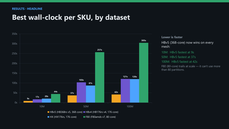
If you are moving Ansys CFX turbomachinery simulation software to the cloud, the first question is not whether Azure can run your computational fluid dynamics (CFD) workloads, but it is which Virtual Machine (VM) delivers the best balance of performance and cost. Azure offers multiple AMD EPYC-based HPC VMs, each optimized differently for compute, memory bandwidth, and price. As a result, the largest VM or the lowest hourly-cost option is not necessarily the most economical choice once the cost of completing a simulation is considered. Ultimately, two metrics matter most: the time to complete a simulation and the cost to run the simulation. To evaluate both, we benchmarked a CFX airfoil case at 10M, 50M, and 100M mesh nodes across Azure HBv5, HBv4, HX, and Fams_v7 VMs. We then validated the optimal HBv5 tuning approach using the TUDA transonic compressor benchmark from TU Darmstadt, a widely recognized open benchmark for turbomachinery CFD. This allowed us to assess whether the observed performance benefits extend beyond a single airfoil test case to a fundamentally different CFD workload. Key findings include: The latest generation HBv5 VM is 2-3x faster than a 176-core node on real meshes, and on any 50M mesh nodes and up it is highly cost effective. On small meshes the economics flip: a 176-core HBv4 delivers the lowest cost per solve. Despite its low hourly cost, Fams_v7 is the most expensive per simulation on large meshes. The TUDA compressor study confirms that the performance benefits seen in the airfoil benchmarks also apply to larger turbomachinery workloads, while smaller models require more careful MPI rank tuning to achieve optimal results. The practical answer to "which VM should I choose?" depends on mesh size and how you run. This guide gives you the crossover points to make that decision with confidence. Benchmark overview The benchmark used an external-aerodynamics airfoil model at 10M, 50M, and 100M mesh nodes. All simulations were performed in single precision using the CPU-based CFX solver. The study evaluated 168 VM, mesh, and rank-count configurations across four Azure VM families and included 254 solver runs, retaining the best result for each configuration. Performance was measured using CFD Solver wall-clock time rather than total workflow runtime. This distinction matters because preprocessing, partitioning, storage, and workflow orchestration overheads vary by environment. Solver wall-clock time isolates the computational workload and provides the clearest view of how each VM family executes and scales CFX. There is also a practical CFX-specific reason to focus on the solver timer. CFX output can report timing for both partitioning and solving, and partitioning is often less sensitive to core count. If users measure the partitioner, scaling may appear artificially flat. The 50M and 100M cases required large partitioning due to 64-bit indexing, while the 10M case used 32-bit indexing. VM Azure family CPU Cores Notes HBv5 HBv5-series EPYC 9V64H Zen 4 cores with HBM 368 High-bandwidth memory for bandwidth-bound HPC HBv4 HBv4-series EPYC 9V33X “Genoa-X” with 3D V-Cache 176 DDR5 with large L3 cache HX HX-series EPYC 9V33X, same as HBv4 176 Larger memory footprint for big models Fams_v7 Fasv7-series, F80ams_v7 EPYC 9005-series "Turin” 80 Compute-optimized general VM Table 1. AMD EPYC-based Azure VM families evaluated in the CFX benchmark. Note: HBv4 and HX share the identical 9V33X CPU, so on compute they are near interchangeable. The primary difference is memory capacity, not speed. Performance comparison The performance story is best seen in the chart below. HBv5 delivered the shortest solver runtime across all three mesh sizes, and its advantage widened as the workload grew. On the 100M-cell model, HBv5 completed the solve in roughly one-third of the time required by HBv4 or HX. Figure 1. Best solver wall-clock time by VM family and mesh size. Lower is faster. Three observations stand out: HBv5 wins every mesh, and its lead widens with size: it is about 2x faster than a 176-core node at 10M, and about 2.9x faster at 100M. HBv4 and HX produced similar solver performance, consistent with their shared AMD EPYC 9V33X processor generation. Fams_v7 showed strong low-rank performance, but it caps at 80 cores and ends up about 7x slower than HBv5 on the 100M mesh. Why cost-per-simulation matters Raw speed and sticker price both mislead in the cloud, because you rent the whole VM by the hour regardless of how many cores a job uses. The metric that governs your bill is cost per completed simulation. Cost per run = solver wall-clock seconds / 3600 x VM hourly rate (Linux, South Central US.) This ties speed and price together, and it is the metric a cloud-adoption business case should be built on. VM $/hr PAYG $/hr 3-yr reserved HBv5 23.76 11.88 HX 10.37 5.18 HBv4 8.64 4.32 Fams_v7 8.47 3.30 Table 2. Azure retail list prices used in the benchmark calculations: Linux, South Central US. VM Airfoil 10M Airfoil 50M Airfoil 100M HBv5 $0.057 $0.242 $0.274 HBv4 $0.041 $0.248 $0.289 HX $0.058 $0.251 $0.345 Fams_v7 $0.104 $0.604 $0.717 Table 3. Cost per solve using PAYG pricing and best solver wall-clock time. Figure 2. Cost to solve the 100M-cell benchmark once. The cost analysis reveals an important shift as model sizes increase. For the smallest 10M mesh case, HBv4 delivers the lowest cost per simulation, despite HBv5 achieving the fastest runtime. However, as workloads grow to 50M and 100M mesh nodes, HBv5 emerges as both the fastest and most cost-effective platform, with its performance advantage more than offsetting the higher hourly VM rate. In contrast, Fams_v7 illustrates the danger of evaluating cloud resources based solely on hourly pricing. While it offers one of the lowest hourly costs, its longer runtimes make it the most expensive option on a per-simulation basis for larger CFD workloads. For organizations running CFX regularly, Reserved Instances can further improve the economics, reducing infrastructure costs by roughly 50% while preserving the same performance characteristics. How CFX scales on Azure HBv5 HBv5 keeps winning as meshes grow because it provides scaling headroom. On the 100M mesh, HBv5 goes from 550 seconds at 16 ranks to 42 seconds at 368 ranks, a 13.2x speed-up, and still gains from higher rank counts at the top of its range. Figure 3. HBv5 scaling for the 100M-cell CFX airfoil benchmark. Fams_v7 can be attractive at very low rank counts, but its scaling is constrained by its 80-core configuration. HBv4 and HX scale to 176 cores before approaching a plateau. HBv5 continues extracting value up to 368 ranks, which is why its advantage grows as models become larger. Transonic compressor validation on HBv5 The TUDA transonic compressor benchmark is selected because it tests the same HBv5 tuning approach on a different physics, i.e., a turbomachinery workload, not just the original airfoil case. The result is consistent: spreading ranks one-per-CCD-first across the 48 CCDs, combined with MPI pinning, helps heavier cases to continue scaling as more of the node is used. Figure 4. TUDA transonic compressor scaling on HBv5 with CCD-spread + MPI pinning. Lower solver wall-clock time is better. This case is a 43M mesh node model and improves from 218 seconds at 48 ranks to 57 seconds at 368 ranks, a 3.8x speed-up, showing that large turbomachinery models have more parallel work available per rank and can keep scaling further up the CCD ladder. Figure 5. Radial Compressor 20M scaling on HBv5 using CCD-spread MPI rank placement. The Radial Compressor 20M benchmark shows the other side of the sizing rule. Solver wall-clock time decreases from 1,173 seconds at 48 ranks to 331 seconds at 368 ranks, a 3.5× reduction in turnaround time, but most of the benefit is captured before the full-node configuration. Above roughly 150–250 ranks the scaling efficiency tapers, because the case is smaller per rank and communication/startup overheads become more visible. This makes the radial-compressor case a useful example: HBv5 still delivers the fastest turnaround, but smaller turbomachinery models should not automatically use every core if cost-per-solve is the goal. Choosing the right Azure VM for your CFX workload The practical rule is to match the VM to the workload rather than to the price tag. For production meshes of roughly 50M mesh nodes and above, HBv5 is the preferred starting point because it offers the strongest combination of turnaround time and cost per completed simulation. For smaller or high-volume short runs around 10M mesh nodes, HBv4 can provide a better cost-per-solve profile. HX should be selected over HBv4 when the additional memory footprint is required, not because compute performance is expected to differ materially. Fams_v7 can be useful for development, sanity checks, or occasional small runs, but it should not be the default production-throughput VM for larger CFX workloads. Users should also validate MPI choice, use large partitioning when required, measure solver time rather than partitioning time, and avoid over-provisioning ranks on small meshes Rule of thumb: The bigger the mesh, the more HBv5 wins on both speed and cost. The smaller the mesh, the more a 176-core HBv4 wins on cost. The crossover in this data sits below the 50M mesh. Practical tuning notes for CFX on Azure VMs Validate MPI choice. MPI performance varied across the Azure VM families tested, with HBv5, HBv4, and Fams_v7 favoring one configuration and HX another. Validate MPI options for your workload and VM configuration. Partition big meshes with -part-large. The 50M and 100M meshes need 64-bit integer indexing, while the 10M mesh runs 32-bit. Measure the solver wall-clock, not the partitioner. CFX output can report total wall-clock time twice: first for partitioning, then for the solver. If scaling looks flat as ranks increase, you may be timing the partitioner. Do not over-provision ranks on small meshes. Tiny cases can hit communication overhead before they use every core. Key takeaways for Azure cloud adoption HBv5 is the preferred platform for production-scale CFX workloads, delivering both the fastest runtimes and the lowest cost per solve on larger meshes. HBv4 remains attractive for smaller workloads where minimizing cost per simulation is more important than minimizing runtime. Cloud sizing decisions should be based on cost per simulation rather than hourly VM pricing. Taken together, Azure gives CFX users a practical cloud-sizing framework: select the VM based on mesh size, solver scalability, and cost per completed simulation. Learn More: Learn more about Ansys CFX capabilities Request a Microsoft Azure Free TrialBuild a Simple GPU-Enabled Kubernetes Cluster on Azure N-Series VMs
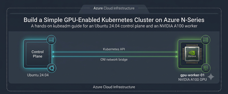
Audience: Platform engineers, ML engineers, and developers who need a small, understandable GPU development cluster without the abstraction of a managed Kubernetes service. Reference topology: Role Azure VM size Operating system Purpose Control plane Standard_D8s_v6 Ubuntu 24.04 LTS API server, scheduler, controllers, etcd GPU worker Standard_NC24ads_A100_v4 Ubuntu 24.04 LTS CUDA-enabled development workloads Software baseline: Kubernetes v1.33, containerd, Flannel CNI, NVIDIA Container Toolkit, and NVIDIA Kubernetes device plugin v0.17.0. Why Build This Cluster? A two-node kubeadm cluster is useful when you want direct access to Kubernetes internals while developing or debugging GPU applications. It keeps the control plane on a general-purpose VM and reserves the expensive N-series capacity for workloads that explicitly request a GPU. Development Use Case: Shared GPU Sandbox Imagine a small ML team validating a PyTorch service before moving it to a production platform. Developers build containers locally or in CI, deploy them to this cluster, request nvidia.com/gpu: 1, inspect CUDA behavior, tune resource requests, and test Kubernetes manifests. The same environment can exercise Jobs, model-serving Deployments, ConfigMaps, Secrets, storage mounts, and observability agents. This design is appropriate for experimentation, integration testing, workshops, and short-lived development. It is not a production blueprint: the control plane is not highly available, etcd has no redundancy, Flannel is intentionally simple, and operational safeguards are minimal. Architecture and Traffic Flow Control plane: runs the Kubernetes API server, scheduler, controller manager, and etcd. GPU worker: runs containerd, kubelet, the NVIDIA container runtime, and GPU workloads. Pod network: Flannel allocates pod addresses from 10.244.0.0/16. GPU discovery: the NVIDIA device plugin advertises nvidia.com/gpu to Kubernetes. Before You Begin Create both VMs in the same Azure virtual network and subnet. Use private IP connectivity between nodes. Confirm that the selected region has quota and capacity for Standard_NC24ads_A100_v4. GPU VM availability and quota are subscription- and region-dependent. Use trusted administrative source ranges for SSH. Ensure the nodes can communicate on the Kubernetes control-plane, kubelet, and Flannel ports required by your network policy. Avoid exposing the Kubernetes API server broadly to the internet. Disk requirement: Use 128GB disk as OS disk in Standard_NC24ads_A100_v4 as 32GB will be the default and it may not be sufficient to run the test job mentioned below. 1. Prepare Both Nodes Run the following commands on both the control-plane VM and the GPU worker. Use a non-root account with sudo access. Set Host Names and Name Resolution Assign a unique host name on each VM: Control plane sudo hostnamectl set-hostname controlplane GPU worker sudo hostnamectl set-hostname gpunode Add both private IP addresses to /etc/hosts on each node, replacing the placeholders: <CONTROL_PLANE_PRIVATE_IP> controlplane <GPU_WORKER_PRIVATE_IP> gpunode Disable Swap Kubelet expects swap to be disabled unless it is explicitly configured to tolerate it. sudo swapoff -a sudo sed -i '/ swap / s/^/#/' /etc/fstab swapon --show The final command should return no active swap devices. Load Required Kernel Modules cat <<EOF | sudo tee /etc/modules-load.d/k8s.conf overlay br_netfilter EOF sudo modprobe overlay sudo modprobe br_netfilter Configure Kubernetes Networking Parameters cat <<EOF | sudo tee /etc/sysctl.d/k8s.conf net.bridge.bridge-nf-call-iptables = 1 net.bridge.bridge-nf-call-ip6tables = 1 net.ipv4.ip_forward = 1 EOF sudo sysctl --system Install and Configure containerd sudo apt-get update sudo apt-get install -y containerd sudo mkdir -p /etc/containerd sudo containerd config default | sudo tee /etc/containerd/config.toml > /dev/null sudo sed -i 's/SystemdCgroup = false/SystemdCgroup = true/g' /etc/containerd/config.toml sudo systemctl restart containerd sudo systemctl enable containerd sudo systemctl status containerd --no-pager The SystemdCgroup = true setting aligns containerd with kubelet and systemd cgroup management. Install Kubernetes v1.33 Packages The repository minor version and the packages installed on every node must match. The commands below configure the v1.33 repository used by this guide. sudo apt-get update sudo apt-get install -y apt-transport-https ca-certificates curl gpg conntrack socat sudo mkdir -p /etc/apt/keyrings curl -fsSL https://pkgs.k8s.io/core:/stable:/v1.33/deb/Release.key | sudo gpg --dearmor -o /etc/apt/keyrings/kubernetes-apt-keyring.gpg echo 'deb [signed-by=/etc/apt/keyrings/kubernetes-apt-keyring.gpg] https://pkgs.k8s.io/core:/stable:/v1.33/deb/ /' | sudo tee /etc/apt/sources.list.d/kubernetes.list sudo apt-get update sudo apt-get install -y kubelet kubeadm kubectl sudo apt-mark hold kubelet kubeadm kubectl kubeadm version kubectl version --client If you choose another supported Kubernetes minor release, replace v1.33 consistently on every node and follow that release’s upgrade and version-skew guidance. 2. Initialize the Control Plane Run this section only on controlplane. Initialize Kubernetes Update the CIDR value as per your requirement sudo kubeadm init --pod-network-cidr=10.xxx.0.0/16 Save the kubeadm join command printed at the end. It contains a time-limited bootstrap token and the control-plane CA hash. Configure kubectl for the Administrator mkdir -p "$HOME/.kube" sudo cp -i /etc/kubernetes/admin.conf "$HOME/.kube/config" sudo chown "$(id -u):$(id -g)" "$HOME/.kube/config" kubectl get nodes The control-plane node may remain NotReady until the CNI is installed. Install Flannel kubectl apply -f https://github.com/flannel-io/flannel/releases/latest/download/kube-flannel.yml kubectl get pods -n kube-flannel -w Because Flannel’s default manifest uses 10.244.0.0/16, it matches the pod CIDR supplied to kubeadm. Generate a New Join Command if Needed kubeadm token create --print-join-command Treat the join command as a secret while it is valid. Run it only on the intended worker. 3. Configure the GPU Worker Complete the shared preparation steps first, then perform the following work on gpunode. Validate the NVIDIA Driver The Azure GPU VM must have a compatible NVIDIA driver. Confirm that the host can see the accelerator: nvidia-smi Do not continue until this command reports the GPU and driver successfully. Driver installation varies by Azure image and extension strategy, so standardize it before automating the node build. Install NVIDIA Container Toolkit curl -fsSL https://nvidia.github.io/libnvidia-container/gpgkey | sudo gpg --dearmor -o /etc/apt/keyrings/nvidia-container-toolkit-keyring.gpg curl -s -L https://nvidia.github.io/libnvidia-container/stable/deb/nvidia-container-toolkit.list | sed 's#deb https://#deb [signed-by=/etc/apt/keyrings/nvidia-container-toolkit-keyring.gpg] https://#g' | sudo tee /etc/apt/sources.list.d/nvidia-container-toolkit.list sudo apt-get update sudo apt-get install -y nvidia-container-toolkit sudo nvidia-ctk runtime configure --runtime=containerd --nvidia-set-as-default sudo systemctl restart containerd sudo systemctl status containerd --no-pager Join the Worker to the Cluster Run the exact command generated by the control plane. It will resemble: sudo kubeadm join <CONTROL_PLANE_PRIVATE_IP>:6443 --token <TOKEN> --discovery-token-ca-cert-hash sha256:<HASH> Back on the control plane, watch the node registration: kubectl get nodes -o wide -w azureuser@controlplane:~$ kubectl get nodes NAME STATUS ROLES AGE VERSION controlplane Ready control-plane 84s v1.33.13 azureuser@controlplane:~$ kubectl get nodes NAME STATUS ROLES AGE VERSION controlplane Ready control-plane 111s v1.33.13 gpunode NotReady <none> 8s v1.33.13 azureuser@controlplane:~$ kubectl get nodes NAME STATUS ROLES AGE VERSION controlplane Ready control-plane 112s v1.33.13 gpunode Ready <none> 9s v1.33.13 4. Advertise the GPU to Kubernetes Run these commands on the control plane. Install the NVIDIA Device Plugin Pinning the manifest version makes the cluster reproducible. curl -fsSL -o nvidia-device-plugin.yml https://raw.githubusercontent.com/NVIDIA/k8s-device-plugin/v0.17.0/deployments/static/nvidia-device-plugin.yml kubectl apply -f nvidia-device-plugin.yml kubectl get daemonset -n kube-system nvidia-device-plugin-daemonset kubectl get pods -n kube-system -l name=nvidia-device-plugin-ds -o wide Verify GPU Capacity kubectl describe node gpunode | grep -A 10 -E 'Capacity:|Allocatable:' kubectl get node gpunode -o jsonpath='{.status.allocatable.nvidia\.com/gpu}{"\n"}' The expected allocatable value depends on the VM’s visible GPU count and partitioning configuration. Kubernetes schedules GPUs as integer extended resources. azureuser@controlplane:~$ kubectl describe node gpunode | grep -A 10 -E 'Capacity:|Allocatable:' Capacity: cpu: 24 ephemeral-storage: 128917488Ki hugepages-1Gi: 0 hugepages-2Mi: 0 memory: 226765912Ki nvidia.com/gpu: 1 pods: 110 Allocatable: cpu: 24 ephemeral-storage: 118810356745 hugepages-1Gi: 0 hugepages-2Mi: 0 memory: 226663512Ki nvidia.com/gpu: 1 pods: 110 System Info: Machine ID: ac82b1424d30473a86a3f22bb2c4ffa1 System UUID: 67d695c2-b663-4514-9952-9e6e29671e4e azureuser@controlplane:~$ kubectl get node gpunode -o jsonpath='{.status.allocatable.nvidia\.com/gpu}{"\n"}' 1 5. Run an End-to-End PyTorch GPU Test Create gpu-test-job.yaml on the control plane with the following content: apiVersion: batch/v1 kind: Job metadata: name: pytorch-gpu-test namespace: default spec: backoffLimit: 2 template: spec: restartPolicy: Never containers: - name: pytorch-trainer image: pytorch/pytorch:2.1.0-cuda12.1-cudnn8-runtime command: ["python3", "-c"] args: - | import time import torch import torch.nn as nn import torch.optim as optim print("=== CUDA validation ===") if not torch.cuda.is_available(): raise SystemExit("CUDA was not detected by PyTorch") device = torch.device("cuda:0") print(f"Device: {torch.cuda.get_device_name(0)}") print(f"Capability: {torch.cuda.get_device_capability(0)}") model = nn.Sequential( nn.Linear(1000, 2048), nn.ReLU(), nn.Linear(2048, 1000) ).to(device) optimizer = optim.SGD(model.parameters(), lr=0.01) criterion = nn.MSELoss() inputs = torch.randn(128, 1000, device=device) targets = torch.randn(128, 1000, device=device) started = time.time() for epoch in range(1, 101): optimizer.zero_grad() loss = criterion(model(inputs), targets) loss.backward() optimizer.step() if epoch % 20 == 0: vram = torch.cuda.memory_allocated(0) / 1e6 print(f"Epoch {epoch}/100 | Loss {loss.item():.4f} | VRAM {vram:.2f} MB") print(f"Completed in {time.time() - started:.4f}s") resources: limits: nvidia.com/gpu: "1" requests: nvidia.com/gpu: "1" Submit and observe the Job: kubectl apply -f gpu-test-job.yaml kubectl get pods -l job-name=pytorch-gpu-test -o wide kubectl logs -l job-name=pytorch-gpu-test --follow kubectl get job pytorch-gpu-test A successful run prints the NVIDIA device name, CUDA capability, training progress, and completion time. azureuser@controlplane:~$ kubectl get pods -l job-name=pytorch-gpu-test -o wide NAME READY STATUS RESTARTS AGE IP NODE NOMINATED NODE READINESS GATES pytorch-gpu-test-j5wh8 1/1 Running 0 109s XXXX gpunode <none> <none> azureuser@controlplane:~$ kubectl logs -l job-name=pytorch-gpu-test --follow === CUDA validation === Device: NVIDIA A100 80GB PCIe Capability: (8, 0) Epoch 20/100 | Loss 1.0461 | VRAM 51.37 MB Epoch 40/100 | Loss 1.0415 | VRAM 51.37 MB Epoch 60/100 | Loss 1.0371 | VRAM 51.37 MB Epoch 80/100 | Loss 1.0328 | VRAM 51.37 MB Epoch 100/100 | Loss 1.0287 | VRAM 51.37 MB Completed in 0.1250s Conclusion This compact cluster provides a transparent path from an Azure GPU VM to a Kubernetes-scheduled CUDA workload. It is small enough to understand, reset, and rebuild, yet realistic enough to validate container images, resource requests, device discovery, Jobs, and model-serving patterns before adopting a production-grade architecture.Retirement of Microsoft HPC Pack
Overview Microsoft HPC Pack is a Windows‑based high‑performance computing (HPC) scheduler that enables customers to deploy, manage, and operate HPC workloads in on‑premises and hybrid environments. Since its original release, HPC Pack has supported a range of Windows‑centric HPC scenarios, including job scheduling, workload orchestration, and integration with Windows Server–based technologies. Microsoft is announcing the planned retirement of HPC Pack. For customers looking to run HPC workloads going forward, Microsoft’s supported platform for managed HPC and parallel workloads is Azure Batch. Customers may also adopt any other Azure service as appropriate for their workload. These platforms provide modern, cloud‑native capabilities for scheduling, scaling, and operating HPC workloads on Azure. Important Dates Retirement announcement: August 27, 2026 End of Support / retirement date: August 27, 2027 After August 27, 2027, HPC Pack will no longer receive feature updates, bug fixes, or standard product support. No new versions or enhancements will be released. Existing HPC Pack deployments will not be forcibly disabled; however, they will be considered unsupported. Support During the Retirement Period HPC Pack is now entering a one-year retirement period that ends at End of Support on August 27, 2027. Microsoft will provide limited, retirement-only support during this period. The scope of this support is defined below so customers know what to expect. What Microsoft will provide during the retirement period: Security response, including investigation of applicable security vulnerabilities (CVEs) and any security updates deemed necessary by Microsoft Guidance based on existing Microsoft documentation, published best practices, and previously validated HPC Pack configurations Assistance with support incidents involving supported HPC Pack components and documented product functionality What is NOT included during the retirement period: Non-security bug fixes Performance, reliability, scalability, or optimization improvements New features or feature enhancements Customer-specific hotfixes, custom code changes, or design modifications Validation or certification of new operating systems, hardware platforms, drivers, firmware, third-party software, or dependencies Validation of new deployment architectures, configurations, or integration scenarios Changes to existing product behavior or design Creation of new documentation, guidance, or troubleshooting content Troubleshooting that requires new product investigation beyond existing product knowledge, documentation, or previously validated scenarios New customer onboarding, solution design, or pre-sales assistance Migration planning, migration execution, or migration consulting services Support for configurations, integrations, or deployment scenarios that are outside published documentation, established best practices, or previously validated HPC Pack environments After End of Support (August 27, 2027): HPC Pack will receive no further updates, fixes, or technical support, and deployments will be considered unsupported. What Customers Should Do Customers currently using HPC Pack should begin planning migration to a supported alternative as soon as possible. For most scenarios, the following services are recommended: Azure Batch – for managed scheduling and execution of parallel and HPC workloads Or any other Azure service as appropriate for your workload Resources HPC Pack documentation: Microsoft HPC Pack 2019 Public issue tracker: Azure/hpcpack GitHub repository Next Steps Customers who anticipate needing additional planning assistance or migration guidance should engage early with their Microsoft account team or Cloud Solution Architect (CSA) to help ensure a smooth transition and avoid potential disruption. To help us understand customer needs and improve future communications, please complete this Microsoft Form. Share any technical, operational, or business challenges you anticipate during your transition. Your feedback will help us identify common concerns and refine future guidance.
Connecting Microsoft Discovery App to Azure HPC with Azure NetApp Files and CycleCloud
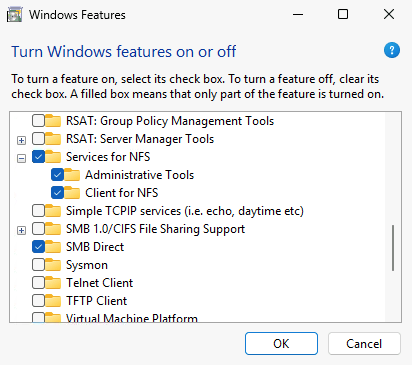
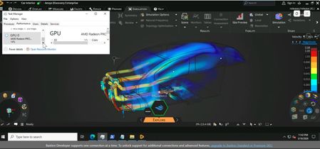
Introduction Traditional High-Performance Computing (HPC) is central to most scientific computing and engineering applications. These systems are based on well tested, repeatable, and scalable compute processes that enable the large-scale generation and validation that the semiconductor and other industries depend on. Integrating AI and agentic flows into this traditional model remains a challenge. Where many agentic systems rely on “modern” compute architecture utilizing REST based communications and object storage, traditional HPC relies on POSIX based file systems and scheduler-based orchestration. Combining these two different disciplines presents a challenge to many engineering and large-scale research enterprises. This blog describes how Microsoft Discovery app can directly interoperate with existing traditional HPC deployments utilizing Azure HPC. Microsoft Discovery is an enterprise agentic AI platform for research and development, designed to help specialized agents reason, plan, execute, and learn in a continuous loop across data, tools, and workflows. It is built on Azure and designed to integrate with capabilities such as Azure HPC and Microsoft Foundry, while leveraging industry proven tools and customer flows, making it a natural bridge between AI-native reasoning and compute-intensive engineering execution. Agentic AI in HPC The value of agentic AI in scientific and engineering workloads is not just as a chatbot or code generator; it is the ability to participate in an existing workflow: write parameter files, launch simulations, inspect logs, summarize failures, generate follow-on jobs, and preserve artifacts for traceability. To do this effectively, agents must be able also read data from POSIX-based file systems and dispatch jobs to the scheduler. To maintain IP security, they must access data while respecting the access limits of the user that dispatched them and write data under the same RBAC rules as that same user. That way organizations can be assured that agents operate strictly under the dispatching user's access rights, so they cannot reach data the user isn't authorized to see and the data they write retains the permissions that the user who dispatches the agent enjoys. Discovery app is currently only available on Windows. Linux and Mac versions will soon be available. In the meantime, enabling the Windows based Discovery app to leverage the capabilities on Azure HPC today with little to no change to the current HPC flow. Reference architecture The architecture has five primary components: a Windows VM running the Discovery app on Azure, an Azure NetApp Files volume that is mounted by both Windows and Linux clients, an Azure CycleCloud-managed HPC cluster with a Linux login node used for job submission and monitoring, and a scheduler that dispatches work to compute nodes. Discovery app on Windows: Runs on a Windows VM placed inside the same VNet, or reachable through controlled private networking, so it can access storage and the login node without exposing the HPC environment publicly. Azure NetApp Files: Provides the shared file namespace for input decks, scripts, logs, generated data, and results. Linux nodes mount the volume with native NFS. Windows can mount the same namespace through the Windows NFS client or an equivalent enterprise file-access solution. Azure CycleCloud: Provisions and manages the HPC cluster, including scheduler, login node, execute nodes, autoscaling, and cluster configuration. Login node: Acts as the controlled command endpoint. Discovery should submit jobs and query scheduler state from here, not run heavy tools directly on the login node. This protects the actual Cyclecloud scheduler and cluster manager from being overwhelmed if the dispatch volume is high. This also allows for scalability if there are many clients scheduling jobs at once. Scheduler: Incumbent schedulers that customers are already using with Azure Cyclecloud handles execution. Discovery creates scripts and submits them through the scheduler so compute runs on the correct nodes with the correct environment, licenses, and policies. This remains the same as how traditional HPC schedules jobs today. Connectivity model Running on a Windows VM in the Azure VNet aligns with many enterprises’ requirement that none of their data or IP can leave their network. Doing this avoids the need to run jobs through a user laptop or unmanaged public endpoint. This also allows the user to start an agentic workload then disconnect from the VM while the job runs and reconnect when they come back. Maintaining the same working model most engineers have with their HPC environment today. For Discovery to access Azure HPC, it needs to map the Azure NetApp Files volumes and command access to the Linux login node. File access lets agents create and read files. Command access lets agents run Linux commands, submit jobs, and monitor execution. Discovery writes execution scripts to the ANF volume, then uses SSH to dispatch the job to the schedule with the execution script. The advantage of this model is that the user can directly provide Unix-style paths to Discovery and tell it to execute tools without the user worrying about being on a Windows platform. For example, CAD teams often provide setup scripts with paths to tools that users are supposed to reference in creating their own tool execution scripts. Using this model, I just tell Discovery to use the setup script /mount/setup/tools/vendora.csh as a template and it will happily find the file and do so. I can then tell Discovery to dispatch the job to the hpc queue and it will schedule to the appropriate SLURM queue where a system is provisioned and assigned to run using the new execution script Discovery creates. This model also gets around the temporary limitation of Discovery app, unlike the enterprise Discovery service, only being available on Windows. In this model, Windows is only acting as a terminal interface so it doesn’t matter that it’s not a platform that normally works with most EDA tools. In fact, users can deploy Discovery app on either x86 or ARM Windows since all the actual tools run on the Linux-based HPC deployment in Azure anyway. Mapping Windows drive to NFS volumes Discovery agents must understand how to access files on the mapped NFS volume from the Windows VM. The same file may appear as Z:\project\run1\exec.csh on Windows and /mount/project/run1/exec.csh on Linux. The skill or instruction file used by Discovery should explicitly describe that mapping and instruct agents to use Linux paths inside batch scripts and scheduler commands. A typical instruction might say: the Windows drive Z: maps to the Linux mount point /mount. If Discovery sees /mount/designs/test.sv, it can read or write the corresponding Windows file at Z:\designs\test.sv. When generating job scripts, it should always use the Linux path, because those scripts run on the cluster. Implementation steps 1. Deploy the HPC foundation Start with the standard Azure HPC foundation: a virtual network, Azure CycleCloud, a scheduler-backed cluster, and shared storage. CycleCloud can deploy and manage Slurm clusters and supports external NFS mounts, including Azure NetApp Files. Configure the cluster so the scheduler and compute nodes mount the shared file system at a stable Linux path such as /mount, /shared, or a customer-specific project path. Make sure that systems can ssh to the login node using a public/private key pair. The login node should be accessible using a command like: % ssh -i .ssh/keyfile user@login-node 2. Place the Windows VM in the same network boundary Create a Windows VM that can reach both the Azure NetApp Files endpoint and the CycleCloud login node over private IP. The required Windows NFS client is available on Windows 11 Pro, Enterprise, and Education. It is not available on Windows 11 Home. Install the Discovery app on that VM. This VM becomes the user’s Discovery workstation for the HPC-connected workflow. Keep the VM inside the same security boundary as the HPC deployment, and use standard enterprise controls such as private networking, restricted inbound access, managed identity where appropriate, and least-privilege SSH keys. 3. Install Microsoft Discovery app Download and install Microsoft Discovery app from: https://github.com/microsoft/discovery Once installed, start Microsoft Discovery app and connect to your Github Copilot account in order to configure access to the LLM AI models. Create a new project 4. Mount the Azure NetApp Files volume into Windows Mount the same shared storage namespace into Windows. The Windows NFS client can map the NFS export to a drive letter such as Z:. The Windows NFS is sufficient for reading logs, results, and data files, and writing execution scripts, parameters, and configuration files. Heavy simulation I/O remain on Linux compute nodes running HPC tools. To configure the Windows NFS Client, you will need to have administrator privileges on your Windows VM. To mount the ANF volume with the Windows NFS client. Press Win+R Run “optional features” Select “More Windows features” Expand “Services for NFS” Enable “Administrative Tools” and “Client for NFS” Click “OK” to install the components. By default, Windows will mount the NFS volume as an anonymous user. To set the correct user, you can define the correct Linux User ID and Group ID in the registry. Note: This is an example of a functional baseline to mount a Linux volume with a user identity as an example. Production environments should employ proper identity mapping for security. Press Win+R Run “regedit” to start the Registry Editor Navigate to HKEY_LOCAL_MACHINE\SOFTWARE\Microsoft\ClientForNFS\CurrentVersion\Default In Default, right click and add two new DWORD entires: AnonymousUID and AnonymousGID Set the values to the decimal value of your Linux UID and GID. This will ensure that you connect to the ANF volume as the correct user. Select OK and then launch the Command Prompt as Administrator. To allow the NFS Client to accept the new registry entries, restart the NFS Client with the following commands: nfsadmin client stop nfsadmin client start Mount the ANF volume to a Windows drive: You should now be able to access your NFS volume by going through the Z: drive. 5. Configure SSH access to the login node Configure the SSH client on the Windows VM with a dedicated key for Discovery-driven access. The key should connect to the CycleCloud login node as the user (same as with NFS above) with permissions to submit jobs, read scheduler state, and access the shared project directory. Verify connectivity by connecting to the Cyclecloud login node using ssh from the Command Prompt. In this example, the username is ai4semi, the IP address of the login node is 10.16.16.25, and the cc_rsa is the keyfile located under the .ssh directory of the user’s home directory on Windows. Since this is the first time for this system to log into the Linux machine, you must accept the connection registration. This will not be necessary for subsequent ssh connects by Discovery using this method. 5. Teach Discovery how to use Azure HPC Now that you have the NFS and SSH connections established in Windows, you simply need to tell Discovery how to use these connections properly to run HPC workloads. In the Discovery chat window, tell Discovery to map the Z: drive on windows to the /mount volume on NFS and how to interact with the files. The Windows drive `Z:` is mapped to the cluster NFS volume `/mount`. - `/mount/<path>` on the cluster corresponds to `z:\<path>` locally. - Example: when a file is referenced as `/mount/test.txt`, look at `z:\test.txt`. Test to make sure Discovery understand by asking it to read a file on the NFS volume using POSIX nomenclature. read the contents of /mount/newfile.txt Discovery should show you the file contents Next, instruct Discovery on how to access and interact with Cyclecloud Connect to the CycleCloud login node over SSH using "ssh -i .ssh\cc_rsa ai4semi@10.16.16.25" Then tell Discovery which scheduler Cyclecloud uses and tell it to check the queue. Cyclecloud is using SLURM as the scheduler. Check the status of the hpc queue. Since the Windows VM is only used to run Discovery and the agentic AI part of the workload and the login node is not meant to run actual HPC workloads, be explicit with Discovery on how it should treat HPC job runs. NEVER run EDA/build/simulation tools on the local system or directly on the login node. ALWAYS submit work to the Slurm scheduler via sbatch. - The login node is for job submission and monitoring only — not for compute. - Wrap every tool invocation in a batch script and submit it with sbatch. 6. Validate the end-to-end workflow Validate that everything works by dispatching a simple test script to Cyclecloud Create a batch script that references the Linux path, submit it to Cyclecloud. dispatch /mount/proj/ai4semi/exec.csh to the hpc queue 7. Save the knowledge for future reference Now that Discovery understands how to access Linux-based files on NFS and how to dispatch jobs, tell it to save the information. Save this knowledge to a skill and use it for all subsequent job runs and file access for the project You see that Discovery now saved the information on how to access files and run jobs to a SKILL.md for general knowledge and updated the copilot-instructions.md to ensure that all subsequent agents and engines understand how to access Azure HPC. Note: These instructions are only scoped to a single project. When creating a new project, you can simply tell Discovery to reach over to your older project to copy the knowledge: copy over instructions on how to access NFS files and paths, and how to dispatch and execute hpc jobs from workspace1 If you want to make this a portable instruction that you can just load for each new project, tell Discovery to create a portable file. package the instructions on how to access NFS files and paths, and how to dispatch and execute hpc jobs into a a single instruction I can provide to new workspaces You can then copy the file to a central location like: C:\Users\ai4semi\project Then for each new project you can tell Discovery to use this file. read and understand the instructions in C:\Users\ai4semi\project\cyclecloud-hpc.instructions.md. Use for all agents and engines in this project and save this information as skills to use in the project Operational considerations Identity and permissions: Keep SSH access scoped to the project and avoid broad administrative privileges. For NFS, verify UID/GID mapping and file ownership behavior before production use. Performance: Use the Windows mount for orchestration artifacts, scripts, and logs. Let Linux compute nodes perform heavy I/O through native ANF mounts. Security: Keep Discovery, storage, and the login node on private networking. Avoid public exposure of scheduler or storage endpoints. Scheduler hygiene: Enforce a rule that Discovery submits jobs through the scheduler and does not run heavy tools interactively on the login node. Conclusion Connecting Microsoft Discovery app to Azure HPC allows users to seamlessly use their existing HPC environment. The most practical approach today is to place Discovery on a Windows VM inside the Azure network, map the shared Azure NetApp Files namespace into both Windows and Linux, and use SSH to submit scheduler-managed jobs through CycleCloud. Using this method, customers can quickly and easily use Discovery to integrate Agentic AI into their current HPC flows. Users can take advantage of AI agents to read and understand specification files, generate code and testbenches based on those specifications, run existing HPC tools on their Azure HPC environment. They can direct Discovery to use the scripts and resources which their CAD teams have developed. Users can create bookshelves by pointing to the documentation directories many tool vendors include in their installations, allowing Discovery to take advantage of documentation which most users don’t have time to fully digest. Over time, native Linux support can reduce the need for Windows-hosted bridging. Until then, this architecture gives teams a secure, and repeatable way to let Discovery agents create, launch, monitor, and learn from real HPC workloads on Azure.Microsoft Discovery: Where HPC meets agentic AI for the next era of EDA
Introduction High-performance computing is the engine behind the most demanding engineering breakthroughs. In electronic design automation, HPC enables massive simulation farms, verification regressions, place-and-route exploration, timing closure, power analysis, and signoff workloads that would be impractical at scale. However, as chip complexity grows, the limiting factor is no longer only compute capacity. It is the ability to reason across enormous design spaces, coordinate specialized tools, preserve engineering context, and decide what to run next. That is where Microsoft Discovery becomes especially interesting. Microsoft Discovery is an enterprise agentic AI platform for research and development, designed to help specialized agents reason, plan, execute, and learn in a continuous loop across data, tools, and workflows. It is built on Azure and designed to interoperate with capabilities such as Azure HPC and Microsoft Foundry, while leveraging industry proven tools and customer flows, making it a natural bridge between AI-native reasoning and compute-intensive engineering execution. The Inflection Point: HPC is required, but not enough Engineering teams already know how to scale compute. They run large regressions, distribute workloads across clusters, burst into cloud capacity, and optimize storage and schedulers around fast-moving design cycles. Yet the harder challenge is often deciding which simulations matter, which failures are related, which tool settings deserve another experiment, and which signals should trigger the next branch of exploration. Traditional HPC gives engineering teams scale. Agentic AI adds accelerated analysis, orchestration, memory, reasoning, and adaptation. The synthesis of the two is not about replacing engineers or replacing EDA tools. It is about turbocharging the engineers by creating an intelligent execution fabric where agents can understand goals, inspect results, choose tools, launch jobs, summarize outcomes, and recommend the next best action. Engineers remain in control of the design intent and final decisions. In this model, the most valuable resource is not compute capacity; it is engineering time. Microsoft Discovery as the agentic layer for engineering R&D Microsoft Discovery focuses on the full R&D lifecycle: knowledge reasoning, code and plan generation, simulation, analysis, and iteration. For semiconductor and EDA workflows, that maps naturally to the way design teams already operate. Timing closure, regression failure, achieving performance targets all require that engineers pour over massive amounts of information from tool run logs, interpret the results based on engineering goals and specifications, and determine how to resolve the gaps. Discovery leverages the same scientific process used in scientific research to help engineers more quickly understand the resulting data, pick out critical learnings, and help compose the next steps and mitigations. Unlike chat interfaces, agents can act and execute specific functions. Agents can be assigned roles: a verification triage agent, a log-analysis agent, a simulation-planning agent, a physical-design exploration agent, a cost-and-capacity agent, or a documentation agent that preserves evidence and rationale. Together, these agents can coordinate around a shared objective and use HPC as the execution and validation vehicle. For semiconductor programs, engineers are the most expensive and constrained part of the process. Every hour spent searching logs, reconciling reports, relaunching routine jobs, copying context between systems, or documenting repetitive findings is an hour not spent on architecture, debug strategy, design tradeoffs, or design sign-off. Discovery’s value is therefore not simply that it can automate tasks; it can help shift engineering effort away from menial coordination work and toward the decisions that improve product outcomes and silicon spins. What this looks like for EDA In a complex silicon project, design teams may run thousands of tests across multiple scenarios, configurations, simulators, and coverage targets. Today, engineers spend significant time reading logs, correlating failures, rerunning jobs, and deciding whether a failure is new, known, flaky, or blocking. Much of that work is necessary, but repetitive. With an agentic workflow, a verification agent could monitor regression output, cluster related failures, inspect logs, identify likely root causes, and propose targeted reruns rather than brute-force rerunning everything. All this helps to provide engineers more time to focus on the work that requires their unique engineering skill and judgement. In physical design, an agentic workflow could help explore constraints, placement strategies, timing violations, congestion hot spots, and power tradeoffs. HPC provides the parallel capacity to run experiments. Discovery-style agent orchestration can help determine which experiments to run, capture why they were run, compare outcomes, and refine the next set of candidates. This provides a guided design-space exploration loop. For signoff and analysis, agents could help connect results across timing, power, reliability, manufacturability, and cost. Instead of treating each report as an isolated artifact, an agentic system can reason across reports, prior runs, known design patterns, and engineering guidance helping to converge faster. Discovery leverages tried-and-true, industry-proven tools to validate the output of AI using the same methods semiconductor teams have relied on for decades. AI can propose code and plans, prioritize validation and simulation, summarize analysis and debug, or recommend next steps, but the validation path still runs through established EDA flows that engineers understand and trust. The Architecture: Agents, Tools, Data, and Compute Discovery’s flow architecture leverages a closed-loop system. Knowledge sources provide context: design specs, prior bugs, regression history, tool documentation, scripts, and engineering notes. Agents reason over that context and formulate next steps. Tool integrations connect those agents to EDA applications, schedulers, storage systems, model endpoints, and analysis pipelines. Azure HPC supplies scalable execution for simulations and compute-heavy analysis. Results flow back into the system so the next decision is better informed than the last. This demonstrates the power of joining agentic AI and HPC. Discovery provides a platform model for coordinating that loop with enterprise expectations around security, governance, transparency, and human oversight. HPC tools provide assurance that the results from AI are valid. Integrating Discovery with Azure HPC for EDA Discovery becomes even more powerful when it is connected to Azure HPC infrastructure purpose-built for compute- and memory-intensive engineering workloads. For EDA, that includes AMD-based Azure HPC virtual machines such as HX-series instances, which are optimized for silicon design and memory-intensive workloads, with large memory capacity, AMD EPYC processors with 3D V-Cache, and high-performance InfiniBand networking. These platforms give agentic workflows the execution fabric needed to run large simulations, regressions, analysis jobs, and design-space exploration at cloud scale for both EDA and other HPC workloads. Storage is equally important. EDA workloads generate and consume enormous numbers of files, and performance often depends on low-latency shared file access as much as raw CPU capacity. Azure NetApp Files provides enterprise-grade file storage for mission-critical HPC and EDA workloads in Azure, giving teams a managed, high-performance storage layer that can support simulation farms, tool installations, design libraries, scratch spaces, and shared project data. Azure NetApp Files also enables customers to use Discovery in a hybrid environment, enabling customers to keep critical data on-prem while using Discovery to optimize cloud-based flows. Many semiconductor teams keep authoritative design data, source repositories, IP libraries, and sign-off environments in on-premises infrastructure. Azure NetApp Files cache volumes can help bridge that workflow by creating a cloud-based cache of active data from an external origin volume. Frequently accessed data can be served close to Azure compute, while the authoritative dataset remains in the existing on-premises design environment. Cluster automation is another important part of enabling the hybrid flow. Azure CycleCloud can help automate the creation, scaling, and lifecycle management of HPC clusters in Azure so teams can stand up cloud capacity around specific EDA workloads rather than manually managing static infrastructure. That is important for agentic workflows because Discovery can reason about what needs to run, determine the proper resources needed, while CycleCloud-backed automation helps ensure the right compute environment is available when those jobs are ready to execute. Just as importantly, hybrid adoption does not need to force customers to replace the scheduling systems their engineering organizations already use. Many semiconductor teams have deep operational investments in incumbent schedulers which CycleCloud already works with, established queues, policies, licenses, scripts, and user workflows. A practical Discovery-plus-Azure-HPC architecture helps bring agentic AI to their existing flows: integrating cloud capacity with existing scheduler patterns, extending familiar job-submission models, and allowing teams to burst selected workloads into Azure while preserving the operational controls that have governed EDA execution for years. In that architecture, Discovery can act as the intelligent orchestration layer across the hybrid estate as well as a productivity accelerator. Agents can reason over design intent, prior results, and engineering context; submit jobs into Azure HPC environments; use AMD-powered compute for demanding EDA runs; access hot data through Azure NetApp Files; and work through cluster automation and scheduler integrations that align with customer operating models. Combined with Azure HPC, Azure NetApp Files helps eliminate storage bottlenecks that can otherwise limit EDA job throughput, allowing compute resources, EDA licenses, and engineering teams to remain productive at scale. The result is a practical synthesis: AI-guided exploration, proven EDA validation, elastic cloud compute, hybrid data access, and scheduler-aware execution that respects the way semiconductor teams already work. Why it matters for semiconductor teams Semiconductor design is a systems problem. Teams must manage more IP, more verification complexity, more software interaction, more foundry requirements, and more pressure to maintain schedules while design sizes and complexity grows. The industry has invested heavily in automation, but much of that automation remains fragmented across scripts, dashboards, job schedulers, and individual expert workflows. The simple fact is that compute is expensive, but engineering time is even more expensive. Improving engineer productivity has an outsized impact on schedule, quality, and cost. Agentic AI offers a way to automation more of the design and verification process. Automating much of the more mechanical parts of the flow. Teams can create workflows that observe, reason, and iterate while agents coordinate the results to achieve the engineering objective. Instead of relying only on tribal knowledge, teams can preserve decisions, evidence, and rationale in a repeatable workflow. Human-in-the-loop by design The goal is not autonomous chip design without engineers. The goal is amplified engineering outcomes. In the most valuable scenarios, agents handle the repetitive, high-volume, evidence-gathering work while engineers define objectives, validate assumptions, approve major decisions, and interpret tradeoffs. Discovery can help reduce the menial burden of searching, summarizing, comparing, rerunning, and documenting so engineers can spend more time on the creative and analytical work only they can do. This is especially important in EDA, where correctness, traceability, and sign-off confidence matter as much as speed. Microsoft Discovery’s emphasis on enterprise governance and transparency is therefore central to the story. In regulated or high-stakes engineering environments, teams need to know what data was used, which tools were invoked, what assumptions were made, and where human approval occurred. Just as important, they need confidence that AI-generated recommendations are validated through established engineering practices, not accepted on faith. Agentic workflows must be auditable, explainable, and grounded in the same EDA verification and signoff discipline the industry already depends on. Conclusion: Going beyond just compute and AI The next phase of EDA acceleration will not come from compute alone, and it will not come from AI alone. It will come from the synthesis of both: HPC infrastructure that can execute at scale, and agentic AI systems that can reason, coordinate, and learn across complex engineering workflows. Microsoft Discovery steps towards that future. For HPC and EDA teams, the opportunity is to move from faster batch execution to intelligent convergence: workflows that know what has been tried, understand what changed, recommend what to try next, and use scalable compute to validate ideas quickly through proven EDA tools and methodologies. In a world where design complexity keeps rising, the ability to combine elastic compute with agentic systems can help to greatly improve productivity, turn repetitive process work into guided automation, and validate AI-assisted decisions through the same trusted engineering practices the semiconductor industry has used for decades. The Microsoft Discovery team will be at Design Automation Conference, July 27-29, 2026, in Long Beach, California. The Microsoft Discovery team will be showcasing how engineers can use agentic AI to enable greater productivity for semiconductor design workloads. Drop by the Microsoft booth (651) to learn more about Microsoft Discovery for semiconductor design. Learn how technologies from AMD and NetApp come together with Azure HPC to provide the high-performance environment for running EDA tools on the cloud.AI Infrastructure Preflight at User space: Validating Multi Node, Multi GPU Slurm Clusters
Every team that operates GPU clusters for AI has seen this pattern. The cluster boots, GPUs are visible, and scheduling works at a basic level. Then the first distributed training run stalls in NCCL initialization, fails during rank rendezvous, or silently maps ranks to the wrong devices. The issue is often not in training code. It is in infrastructure consistency across scheduler, runtime, drivers, networking, and process topology. The goal of ai-infra-validator is straightforward: Run a fast user space preflight before expensive training jobs. Validate distributed initialization for multi node, multi GPU workloads. Confirm GPU affinity and rank mapping are correct. Verify NCCL communication fabric can complete a collective ring under Slurm. This post walks through the implementation in detail, explains why each part exists, and shows how to operationalize it in real HPC AI environments. What the project validates Zero-dependency user space smoke test for AI clusters. Validates multi-node PyTorch DDP initialization, GPU affinity, and NCCL fabric connectivity under Slurm orchestration. Git Repo: ai-cluster-validator In practical terms, this checks that: Slurm launches the expected number of ranks per node. Distributed process group creation with NCCL succeeds. Each rank binds to the expected local GPU. Cross-rank all-reduce completes and converges. Node level telemetry confirms software and fabric state. This is not a performance benchmark. It is a correctness and readiness gate. Tested platform profile Component Value CycleCloud 8.8.3-3667 Slurm 25.05.5 Slurm partition hpc Scheduler VM SKU Standard_D8s_v6 Compute VM SKU Standard_ND96asr_v4 OS images microsoft-dsvm:ubuntu-hpc:2204:latest and microsoft-dsvm:ubuntu-hpc:2404:latest PyTorch 2.12.0+cu130 CUDA runtime 13.0 NCCL target 2.29.7 This profile represents a common enterprise scenario where scheduler and compute nodes have different roles, and the training fleet depends on correct multi node orchestration. Step 1: Minimal user space bootstrap The bootstrap script creates a shared Python environment at /shared/apps/pytorch_env and installs the required packages: torch torchvision torchaudio psutil This choice is intentional: No dependency on containers for first-pass validation. Single environment path visible to all compute nodes. Rapid setup and repeatability for cluster operators. Command sequence: git clone https://github.com/vinil-v/ai-cluster-validator.git cd ai-cluster-validator sudo bash bootstrap_env.sh Step 2: Slurm job defines deterministic distributed topology The Slurm script expresses a clear topology contract: nodes=2 ntasks-per-node=8 gpus-per-node=8 cpus-per-task=12 From this, world size is derived as: WORLD_SIZE = SLURM_NTASKS = 2 x 8 = 16 The script also configures network and NCCL behavior: NCCL_DEBUG=WARN NCCL_IB_DISABLE=0 NCCL_P2P_DISABLE=0 NCCL_IGNORE_CPU_AFFINITY=1 GLOO_SOCKET_IFNAME=eth0 NCCL_SOCKET_IFNAME=eth0 Important implementation detail: MASTER_ADDR is set to the first host in SLURM_JOB_NODELIST. MASTER_PORT is selected dynamically from the ephemeral range 49152-65535 and falls back to 29500 if needed. Why this matters: Reduces port collision risk when jobs run frequently. Avoids hardcoded rendezvous values that may fail in shared clusters. Launch path: srun --cpu-bind=none bash -c " source /shared/apps/pytorch_env/bin/activate; export RANK=$SLURM_PROCID; export LOCAL_RANK=$SLURM_LOCALID; python3 ddp_mesh_ping.py " The LOCAL_RANK handoff is critical for stable GPU affinity inside each node. Step 3: DDP initialization and rank to GPU affinity Inside ddp_mesh_ping.py, each process executes: Parse WORLD_SIZE, RANK, LOCAL_RANK, MASTER_ADDR, MASTER_PORT. Initialize torch.distributed with backend nccl and TCP init method. Set CUDA device using LOCAL_RANK. Core initialization path: dist.init_process_group( backend="nccl", init_method=f"tcp://{master_addr}:{master_port}", world_size=world_size, rank=rank ) torch.cuda.set_device(local_rank) This validates the minimum distributed contract required by real model training jobs. Step 4: Rich node and fabric telemetry in user space Each rank collects detailed metadata before the collective test: Node identity from Slurm and hostname. GPU model and VRAM from CUDA properties. System memory via psutil. CPU model from /proc/cpuinfo. OS and kernel versions. NVIDIA driver version from /proc/driver/nvidia/version. PyTorch, CUDA, and NCCL runtime versions. InfiniBand device state and link rate from /sys/class/infiniband. Basic GPU peer access capability via torch.cuda.can_device_access_peer. All rank payloads are gathered on rank 0 using dist.gather_object and printed as: Cluster hardware topology report. Node environment deep dive. Network interconnect and fabric status. This design gives platform teams one artifact that is both operational and diagnostic. Step 5: Functional collective validation After telemetry, each rank executes a lightweight DDP compute path: Build nn.Linear(10,10) on local GPU. Wrap with DistributedDataParallel. Perform forward, loss, backward. Run all_reduce on loss tensor. Compute global average loss. Pass condition is explicit in log output: SUCCESS: DDP Multi-Node AllReduce Ring Complete! This confirms that process group initialization and collective communication both completed successfully. What a successful run looks like Submission: sbatch ddp_smoke_test.slurm squeue Representative outcomes in the log: Total Execution Ranks: 16 Two nodes with local ranks 0 through 7 on each node GPU inventory aligned with expected A100 topology Active InfiniBand HCAs discovered per host NCCL socket interface set to eth0 Final success marker and computed convergence loss When these markers are present and coherent with expected hardware shape, the cluster is typically ready for distributed training bring-up. How to check the output file The Slurm script writes two artifacts per job: ai_infra_smoke_test_<jobid>.log ai_infra_smoke_test_<jobid>.err Use this exact workflow after submission: # 1. Submit and capture the job id sbatch ddp_smoke_test.slurm # 2. Check job state squeue -j <jobid> # 3. Read standard output log cat ai_infra_smoke_test_<jobid>.log # 4. Read standard error log cat ai_infra_smoke_test_<jobid>.err For stronger validation in automation, also check: Total Execution Ranks equals expected world size. Both nodes appear in the topology table with local ranks 0 through 7. NCCL/CUDA/PyTorch versions are present in the node environment section. Complete reference output Use the following full log as a known-good reference from a successful 2-node ND96asr_v4 run. Master Node IP/Hostname: ddpcluster-hpc-1 Dynamically Assigned Port: 53593 Total Execution Ranks: 16 =============================================================================================== HPC CLUSTER INTERACTION MONITOR =============================================================================================== --> Initializing DDP on Master Node : ddpcluster-hpc-1 --> Dynamic Coordination Port : 53593 --> Target World Cluster Size : 16 GPUs ----------------------------------------------------------------------------------------------- =============================================================================================== CLUSTER HARDWARE TOPOLOGY REPORT =============================================================================================== | Rank | Node Name | Local ID | GPU Model | VRAM | Sys Mem | CPU Cores | ----------------------------------------------------------------------------------------------- | 0 | ddpcluster-hpc-1 | 0 | NVIDIA A100-SXM4-4 | 39.5 GB | 885.8 GB | 96 Cores | | 1 | ddpcluster-hpc-1 | 1 | NVIDIA A100-SXM4-4 | 39.5 GB | 885.8 GB | 96 Cores | | 2 | ddpcluster-hpc-1 | 2 | NVIDIA A100-SXM4-4 | 39.5 GB | 885.8 GB | 96 Cores | | 3 | ddpcluster-hpc-1 | 3 | NVIDIA A100-SXM4-4 | 39.5 GB | 885.8 GB | 96 Cores | | 4 | ddpcluster-hpc-1 | 4 | NVIDIA A100-SXM4-4 | 39.5 GB | 885.8 GB | 96 Cores | | 5 | ddpcluster-hpc-1 | 5 | NVIDIA A100-SXM4-4 | 39.5 GB | 885.8 GB | 96 Cores | | 6 | ddpcluster-hpc-1 | 6 | NVIDIA A100-SXM4-4 | 39.5 GB | 885.8 GB | 96 Cores | | 7 | ddpcluster-hpc-1 | 7 | NVIDIA A100-SXM4-4 | 39.5 GB | 885.8 GB | 96 Cores | | 8 | ddpcluster-hpc-2 | 0 | NVIDIA A100-SXM4-4 | 39.5 GB | 885.8 GB | 96 Cores | | 9 | ddpcluster-hpc-2 | 1 | NVIDIA A100-SXM4-4 | 39.5 GB | 885.8 GB | 96 Cores | | 10 | ddpcluster-hpc-2 | 2 | NVIDIA A100-SXM4-4 | 39.5 GB | 885.8 GB | 96 Cores | | 11 | ddpcluster-hpc-2 | 3 | NVIDIA A100-SXM4-4 | 39.5 GB | 885.8 GB | 96 Cores | | 12 | ddpcluster-hpc-2 | 4 | NVIDIA A100-SXM4-4 | 39.5 GB | 885.8 GB | 96 Cores | | 13 | ddpcluster-hpc-2 | 5 | NVIDIA A100-SXM4-4 | 39.5 GB | 885.8 GB | 96 Cores | | 14 | ddpcluster-hpc-2 | 6 | NVIDIA A100-SXM4-4 | 39.5 GB | 885.8 GB | 96 Cores | | 15 | ddpcluster-hpc-2 | 7 | NVIDIA A100-SXM4-4 | 39.5 GB | 885.8 GB | 96 Cores | =============================================================================================== NODE ENVIRONMENT DEEP DIVE ----------------------------------------------------------------------------------------------- [ddpcluster-hpc-1] Details: --> CPU Microarchitecture : AMD EPYC 7V12 64-Core Processor --> Operating System : Ubuntu 22.04.5 LTS --> Kernel Base Version : 5.15.0-1110-azure --> Nvidia Driver Loaded : 580.126.20 --> PyTorch Environment : v2.12.0+cu130 --> CUDA Runtime Version : v13.0 --> NCCL Fabric Target : v2.29.7 --> Discovered InfiniBand HCAs: - mlx5_an0:1 (4: ACTIVE - 40 Gb/sec (4X QDR)) - mlx5_ib0:1 (4: ACTIVE - 200 Gb/sec (4X HDR)) - mlx5_ib1:1 (4: ACTIVE - 200 Gb/sec (4X HDR)) - mlx5_ib2:1 (4: ACTIVE - 200 Gb/sec (4X HDR)) - mlx5_ib3:1 (4: ACTIVE - 200 Gb/sec (4X HDR)) - mlx5_ib4:1 (4: ACTIVE - 200 Gb/sec (4X HDR)) - mlx5_ib5:1 (4: ACTIVE - 200 Gb/sec (4X HDR)) - mlx5_ib6:1 (4: ACTIVE - 200 Gb/sec (4X HDR)) - mlx5_ib7:1 (4: ACTIVE - 200 Gb/sec (4X HDR)) ----------------------------------------------------------------------------------------------- [ddpcluster-hpc-2] Details: --> CPU Microarchitecture : AMD EPYC 7V12 64-Core Processor --> Operating System : Ubuntu 22.04.5 LTS --> Kernel Base Version : 5.15.0-1110-azure --> Nvidia Driver Loaded : 580.126.20 --> PyTorch Environment : v2.12.0+cu130 --> CUDA Runtime Version : v13.0 --> NCCL Fabric Target : v2.29.7 --> Discovered InfiniBand HCAs: - mlx5_an0:1 (4: ACTIVE - 40 Gb/sec (4X QDR)) - mlx5_ib0:1 (4: ACTIVE - 200 Gb/sec (4X HDR)) - mlx5_ib1:1 (4: ACTIVE - 200 Gb/sec (4X HDR)) - mlx5_ib2:1 (4: ACTIVE - 200 Gb/sec (4X HDR)) - mlx5_ib3:1 (4: ACTIVE - 200 Gb/sec (4X HDR)) - mlx5_ib4:1 (4: ACTIVE - 200 Gb/sec (4X HDR)) - mlx5_ib5:1 (4: ACTIVE - 200 Gb/sec (4X HDR)) - mlx5_ib6:1 (4: ACTIVE - 200 Gb/sec (4X HDR)) - mlx5_ib7:1 (4: ACTIVE - 200 Gb/sec (4X HDR)) ----------------------------------------------------------------------------------------------- NETWORK INTERCONNECT & FABRIC STATUS ----------------------------------------------------------------------------------------------- --> Target Communication Interface (NCCL_SOCKET_IFNAME) : eth0 --> Active Telemetry Tracking Level (NCCL_DEBUG) : WARN --> Inter-GPU Topo Link Verification : Active (P2P/NVLink Capable) ----------------------------------------------------------------------------------------------- SUCCESS: DDP Multi-Node AllReduce Ring Complete! --> Computed System Verification Convergence Loss : 1.398719 =============================================================================================== Why this is effective for platform operations For AI infrastructure teams, this pattern is highly effective because it is: Fast: can be run after every change window. Deterministic: same topology contracts every run. Actionable: output includes enough context for first-level triage. Low friction: user space only, no heavy control plane dependencies. This supports common operating workflows: Day-0 cluster acceptance. Day-1 patch validation after driver, kernel, or image changes. Regression gate in golden image pipelines. Preflight before large multi node model training jobs. Practical guidance for extending to larger clusters Adjust Slurm directives for nodes and tasks per node. Keep one rank per GPU unless validating alternate placement policy. Set NCCL_SOCKET_IFNAME and GLOO_SOCKET_IFNAME according to your network policy. Preserve the dynamic MASTER_PORT logic to avoid static collisions. Keep the success marker string stable so automation can parse it. Closing perspective Most distributed training failures are expensive because they are discovered late. A user space preflight that validates scheduler topology, rank rendezvous, GPU affinity, and NCCL collectives provides a high value guardrail before production starts. ai-infra-validator is a practical implementation of that guardrail. It is compact, transparent, and aligned with how real Slurm based AI clusters operate. For teams running multi node multi gpu training at scale, this kind of preflight should be a standard operational gate.
Distributing model weights to your AI cluster: a faster pre-flight on AKS and Slurm
Standing up an N-node training or inference job and waiting forever for the model checkpoint to land on every node's NVMe? Here's a small Rust + MPI tool — azcp-cluster — that pays Azure egress once, broadcasts over your fabric, and finishes in seconds. Plus the AKS and Slurm patterns to wire it into a real pipeline.Simplify troubleshooting at scale - Centralized Log Management for CycleCloud Workspace for Slurm
Training large AI models on hundreds or thousands of nodes introduces a critical operational challenge: when a distributed job fails, quickly identifying the root cause across scattered logs can become incredibly time-consuming. This manual process delays recovery and reduces cluster utilization. The ability to quickly parse centralized cluster logs from a single interface is critical to ensure job failure root cases are swiftly identified and mitigated to maintain high cluster utilization. Solution Architecture This is a turnkey, customizable log forwarding solution for CycleCloud Workspace for Slurm that centralizes all cluster logs into Azure Monitor Logs Analytic. The architecture uses Azure Monitor Agent (AMA) deployed on every VM and Virtual Machine Scale Set (VMSS) to stream logs defined by Data Collection Rules (DCR) to dedicated tables in a Log Analytics workspace where they can be queried from a single interface. The turnkey solution captures three categories of logs essential for troubleshooting distributed workloads, but can be extended for any other logs: Slurm logs including slurmctld, slurmd, etc., plus archived job artifacts (job submission scripts, environmental variables, stdout/stderr) collected via prolog/epilog scripts. Infrastructure logs including those from CycleCloud including the CycleCloud Healthagent which automatically tests nodes for hardware health and draining nodes that fail tests. Operation System logs from syslog and dmesg capturing kernel events, network state changes, and hardware issues. Each log source flows through its own DCR into a dedicated table following a consistent schema. The solution automatically associates scheduler-specific DCRs with the Slurm scheduler node and compute-specific DCRs with compute nodes handling dynamic node scaling transparently. The solution is purpose-built for CycleCloud Workspace for Slurm, but designed in a modular fashion to be easily extended for new data sources (i.e. new log formats) and processing (i.e. Data Collection Rules) to support log forwarding and analysis of other required logs. Key Benefits Time-series correlation: Azure Monitor's time-based indexing enables rapid identification of cascading failures. For example, trace a network carrier flap detected in syslog to corresponding slurmd communication errors to specific job failures all within seconds. Centralized visibility: Query logs from thousands of nodes through a single interface instead of SSH-ing to individual machines. Correlate Slurm controller decisions with node-level errors and system events in one query. Log persistence: Logs survive node deallocations and reimaging. Critical in cloud environments where compute nodes are ephemeral. Powerful query language: KQL (Kusto Query Language) allows parsing raw logs into structured fields, filtering across multiple sources, and building operational dashboards. Example queries detect patterns like repeated job failures, network instability, or resource exhaustion. Production-ready scalability: User-assigned managed identities automatically propagate to new VMSS instances, and DCR associations handle thousands of nodes without manual configuration. Getting Started The complete solution is available on GitHub (slurm-log-collection) with deployment scripts that: Create all required Log Analytics tables Deploys pre-configured DCRs for Slurm, CycleCloud, and OS logs Automatically associate DCRs with scheduler and compute resources After configuring environment variables and running the setup scripts, logs begin flowing to Azure Monitor and will populate within 15 minutes, but normal log ingestion latency is ~30s to 3 minutes. The repository includes sample KQL queries for common troubleshooting scenarios to accelerate time-to-resolution and to perform non-troubleshooting analysis of cluster usage.