analytics
117 Topics
Optimize selective analytics reads in Azure Data Lake Storage with ABFS Vectored Read
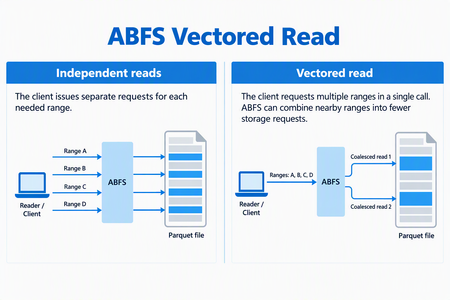
ABFS Vectored Read helps compatible analytics engines reduce request overhead when reading selected portions of columnar files in Azure Data Lake Storage. By coordinating multiple noncontiguous byte ranges through the Azure Blob File System (ABFS) driver, it can combine nearby ranges into fewer storage requests and execute those requests asynchronously. For data engineers working with selective Parquet queries, this brings the storage read pattern closer to what the query needs: a coordinated set of ranges rather than a collection of independent small reads. When the Parquet reader supports vectored I/O and the runtime includes a compatible ABFS client, Spark workloads that use higher-level APIs can enable this capability through configuration - without rewriting queries, changing application logic, or migrating data. Why selective reads need coordinated I/O Consider a query that selects a few columns from a Parquet dataset and filters out most row groups. The reader can skip much of the data the query doesn't need, but the data it needs may be spread across different parts of the file. Reading each range independently can create many small storage requests. Each request carries network and processing overhead, so selecting less data doesn't necessarily remove the cost of coordinating those reads. Vectored Read lets a compatible reader provide the ranges together, giving the client an opportunity to plan the I/O as a group. How ABFS Vectored Read works A compatible reader submits the file ranges it needs together. ABFS validates and sorts the ranges, combines nearby ranges when appropriate, and divides the resulting work to fit its read buffers. It then queues the storage requests asynchronously and returns the requested bytes to the corresponding range buffers. Illustrative request pattern, not a benchmark. Actual grouping depends on range layout and client configuration; coalesced storage requests can include bytes between the requested ranges. This is a client-side optimization. It does not change the file format or rewrite your stored data. The engine still receives the data for the ranges it requested. What this means for your workloads For compatible selective-read workloads, Vectored Read offers: Less request overhead: Combining nearby ranges can reduce separate storage requests and network round trips. Coordinated I/O: Asynchronous reads allow the client to work on multiple requested ranges without treating every range as an isolated operation. Configuration-based adoption: Compatible Spark workloads using the Hadoop Parquet and ABFS path can use the feature without rewriting their queries. The best starting point is a workload that reads selected portions of Parquet files through abfs:// or abfss://. Full sequential scans may see less benefit, and engines that bypass the Hadoop/ABFS path do not use this capability. Support depends on the Hadoop, hadoop-azure, and parquet-hadoop libraries included in the runtime, not only on the Spark version. See Availability and resources for the minimum versions and verification guidance. The benefit depends on the number, size, and spacing of requested ranges, the coalescing configuration, storage and network latency, concurrency and caching. Combining ranges can reduce requests and round trips, but it can also read additional bytes between noncontiguous requested ranges. Compare query duration, storage transactions, bytes read, and resource utilization against a controlled baseline using representative data and concurrency. Get started First, verify that your runtime contains Apache Hadoop 3.3.5 or later, including the hadoop-azure module, and parquet-hadoop 1.12.3 or later. The presence of an ABFS URI alone does not establish that the optimized implementation is installed. For Spark, enable the Parquet setting before the application starts, using the spark.hadoop. prefix: spark-submit \ --conf spark.hadoop.parquet.hadoop.vectored.io.enabled=true \ <other-options> \ <application> Replace the command placeholders with your normal submission options and application. Set the property explicitly rather than relying on a default, which can vary by packaged Parquet version. For managed services, use the service's supported cluster or session configuration mechanism. Availability and resources Azure Databricks does not currently support ABFS Vectored Read because its runtime ships an ABFS version that does not include this capability. In addition, Photon does not use the ABFS driver for data access, even when a workload uses an abfs:// or abfss:// URI. Therefore, the presence of an ABFS URI alone does not indicate that Vectored Read is available. For other packaged or managed runtimes, verify that the environment includes Apache Hadoop 3.3.5 or later with the hadoop-azure module, and parquet-hadoop 1.12.3 or later. Start with one representative selective-read workload and compare it with your baseline. For background, see the ABFS driver overview.142Views1like0CommentsMigrating Azure Cosmos DB Across Regions
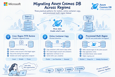
What this article delivers? A decision-oriented, implementation-ready walkthrough based on a hands-on Azure Cosmos DB for NoSQL lab. It corrects the online copy sequence, includes the required Azure CLI snippets, and separates migration duration from application cutover downtime. Regional migration in Azure Cosmos DB is not a single operation. The correct pattern depends on whether the priority is the simplest supported move, the smallest application outage, or a durable multi-region architecture. The Three Migration Patterns at a Glance Pattern Best fit App impact Destination Primary caution 1. Cross-Region PITR restore Simplest regional move Stop writes during final cutover New account created by restore Target-region capacity and restore-point readiness 2. Online copy Minimal downtime Source stays online until cutover Pre-created account and empty target containers Preview prerequisites, RBAC, RU limits, one job per container 3. Provisioned multi-region HA/DR and predictable throughput Online while adding region; controlled failover Same account, second region Higher ongoing cost; conversion back to serverless is not a standard self-service path Before you migrate: establish the decision inputs A reliable migration plan starts by separating total data-movement time from business downtime. Online copy can run for hours or days without requiring the application to stop. Restore may complete quickly, but the application still needs a controlled write freeze, validation, endpoint change, and restart. Define both measures explicitly. Capacity is a migration dependency: A restore that creates a new account still requires the target region to accept the deployment. Validate region availability early, keep an escalation path ready, and avoid treating a successful small-environment test as a capacity guarantee for production. Current Environment Setup Cosmos DB Environment with Capacity Mode= Serverless: Current CosmoDB Topology: Data Count in current database pre-migration: Approach 1: Cross-region point-in-time restore This is the preferred first option when the customer can accept a short write outage and is comfortable moving to a new Cosmos DB account. The restore operation creates the target account; you do not pre-create the destination account as you do for online container copy. Conceptual Plan: Execution flow Confirm the source account uses continuous backup and that the required restore point is available. Validate target-region readiness and prepare the target account name, resource group, networking, identity, and application configuration plan. Schedule the cutover and stop application writes. Start the restore into the target region. Azure creates the new account. Validate account state, databases, containers, policies, item counts, networking, private endpoints, and data-plane RBAC. Update the application endpoint and credentials or managed-identity assignments. Start the application and validate reads and writes. Keep the source account unchanged for an agreed rollback window, then retire it after sign-off. Pre-checks and validation snippets RG="CosmoDB_Demo" SRC_ACCOUNT="demotestingenvironment" az cosmosdb show \ --resource-group "$RG" \ --name "$SRC_ACCOUNT" \ --query "{Account:name,BackupPolicy:backupPolicy.type,Locations:locations[].locationName,State:provisioningState}" \ -o json Review BackupPolicy Type: Note Follow Restore an Account That Uses Continuous Backup Mode - Azure Cosmos DB | Microsoft Learn to update to restore option In the Azure Portal: Cosmos DB → testingenvironmentfordemo → Backup & Restore. Periodic → Continuous Referesh the page and fill in Restore requirements. Cross region restore incurs additional charges on top of the normal point-in-time restores, the price depends on the regions that you are restore from and to. Learn more New Account is created, with data: Testing and Validation Check if the deployment is successful: Count of data across both databases are the same: Approach 2: Online container copy with minimal downtime Online container copy is a container-by-container migration. The application continues reading and writing to the source during the initial copy and incremental synchronization. At cutover, the team stops source writes, waits for the job to catch up, calls the completion operation, validates the target, and then switches the application. The Azure CLI command group and the feature are preview capabilities, so production adoption should include preview acceptance, current limitation review, and a tested fallback. Reference topology used in the lab Component Source Destination Account demotestingenvironment demotestingenvironmentrestore Database demotestingDB demotestingDB Container demotestingDBID demotestingDBID-copy Partition key /category /category Mode Serverless Serverless in the lab Step 1: Define reusable variables RG="CosmoDB_Demo" SRC_ACCOUNT="demotestingenvironment" DEST_ACCOUNT="demotestingenvironmentrestore" SRC_DB="demotestingDB" SRC_CONTAINER="demotestingDBID" DEST_DB="demotestingDB" DEST_CONTAINER="demotestingDBID-copy" JOB="online-copy-hls-final-04" Install the copy extension az extension add --name cosmosdb-preview --upgrade Step 2: Verify source az cosmosdb show -g "$RG" -n "$SRC_ACCOUNT" --query "{Backup:backupPolicy.type,Capabilities:capabilities[].name,State:provisioningState}" -o json Confirm that Backup is Continuous. Confirm that the source has All Versions and Deletes change feed enabled, and review compatibility limitations before applying the capability to an existing production account. Step 3: Create the empty destination container az cosmosdb sql container create -g "$RG" -a "$DEST_ACCOUNT" -d "$DEST_DB" -n "$DEST_CONTAINER" -p "/category" Configure source identity and destination access az cosmosdb identity assign -g "$RG" -n "$SRC_ACCOUNT" SRC_PRINCIPAL=$(az cosmosdb show -g "$RG" -n "$SRC_ACCOUNT" --query "identity.principalId" -o tsv) az cosmosdb update -g "$RG" -n "$SRC_ACCOUNT" --default-identity "SystemAssignedIdentity" az cosmosdb sql role assignment create -g "$RG" -a "$DEST_ACCOUNT" --role-definition-id "00000000-0000-0000-0000-000000000002" --principal-id "$SRC_PRINCIPAL" --scope "/" Step 4: Start Online Copy az cosmosdb copy create --resource-group "$RG" --job-name "$JOB" --src-account "$SRC_ACCOUNT" --dest-account "$DEST_ACCOUNT" --src-nosql database="$SRC_DB" container="$SRC_CONTAINER" --dest-nosql database="$DEST_DB" container="$DEST_CONTAINER" --mode Online Monitor az cosmosdb copy show -g "$RG" -a "$DEST_ACCOUNT" -n "$JOB" --query "{Status:status,Processed:processedCount,Total:totalCount,Error:error}" -o table Query the destination container SELECT * FROM c WHERE c.id = "HLS-ONLINE-COPY-001" Also review via CLI The record appearing in the destination proves both the initial copy and the incremental-change path. Also compare source and target counts, but do not rely on count equality alone; validate representative documents, partition-key values, updates, deletes, TTL behavior, and application queries. Note: Perform the production cutover correctly Stop all writes to the source container. Wait for the online job to catch up and confirm Error is null. Run the complete operation to finalize the online copy job. Validate target counts, representative records, updates/deletes, indexing behavior, networking, identity, and application connectivity. Switch the application endpoint to the destination account and container. Run read/write smoke tests and monitor 429s, 403s, latency, and error rates. Keep the source unchanged for the approved rollback window, then retire it. Approach 3: Convert to provisioned throughput and use multi-region replication This pattern changes the question from “How do I copy data into a second account?” to “How do I extend the existing account into a second region and fail over?” It is appropriate when the workload needs predictable throughput, stronger regional resiliency, or serverless limits make copy-based approaches impractical. Convert the existing serverless account to provisioned throughput. Review and right-size the initial manual throughput assigned to each container or database. Add the target region as an additional region on the same account. Wait for replication and validate application connectivity. Change failover priority or initiate the approved failover method so the target region becomes the write region. Decide whether to retain the original region for HA/DR or remove it after validation. Convert: Azure Portal → Cosmos DB → demotestingenvironment → Overview → Change capacity mode to provisioned throughput and confirm. Refresh and the capacity mode should change. Under Settings, select Replicate data globally, Select West US 2 as the existing region and under Additional regions, select North Central US. Change the write region: Validate current write region Decision framework Decision question Restore Online copy Provisioned multi-region Can the app stop writes briefly? Best fit Not required during bulk copy Not required while adding region Must the target be an existing account? No; restore creates a new account Yes; pre-create target account/container Same account Need to remain serverless? Supported if target deployment is accepted Possible, but throughput can slow copy No; account becomes provisioned Need built-in regional HA after migration? Single target account unless redesigned Single target account unless redesigned Best fit Main production risk Target capacity and cutover validation Preview prerequisites, RBAC, 429s, copy duration Cost, throughput sizing, irreversible architecture choice References Container Copy Jobs - Azure Cosmos DB Azure CLI: az cosmosdb copy Restore an Azure Cosmos DB account using continuous backup Migrate an account to continuous backup mode Configure data-plane role-based access control Change from serverless to provisioned throughput Compare provisioned throughput and serverless Azure Cosmos DB pricing218Views1like0CommentsOptimizing Oracle-to-Power BI Performance and the Path to Modern Analytics
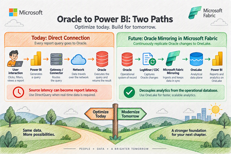
Organizations frequently rely on Oracle databases for large-scale operational workloads while using Microsoft Power BI as their enterprise analytics and visualization platform. Although connecting Power BI directly to Oracle is fully supported, performance can become challenging as datasets grow into the millions of rows. A recent enterprise scenario involving millions of Oracle records illustrates an important principle: Oracle-to-Power BI performance should not be attributed to a single component without first isolating the entire retrieval path. This article provides a practical framework for optimizing that architecture today, while also examining how Microsoft Fabric Mirroring can provide a different data-access pattern for future analytics workloads. The Performance Challenge Consider an Oracle environment containing approximately 15 million records. Testing showed substantially different behavior depending on the client used to retrieve the same Oracle data: A direct Oracle query executed through TOAD returned millions of rows in about eight minutes. Tableau connected to the same Oracle table from the same laptop and refreshed millions of rows in 20 to 30 minutes. Power BI Desktop, however, continued processing for multiple hours before the operation was terminated by network or database controls. Importantly, the Power BI query did not contain additional Power Query transformations. The customer was directly executing SQL and loading the resulting data. This is an extremely useful diagnostic comparison because it demonstrates that Oracle is capable of returning the underlying dataset considerably faster than the Power BI test. It does not, however, prove that the Power BI Oracle connector itself is the single root cause. Performance Is a Pipeline, Not a Single Component Oracle-to-Power BI performance involves several layers: A bottleneck at any one of these layers can affect overall refresh or query performance. Therefore, the first architectural principle is: Measure every layer before attempting to tune the entire solution. A troubleshooting exercise should evaluate: Oracle server-side execution time SQL execution plan Oracle provider/client behavior FetchSize behavior Network transfer Power Query evaluation Query folding Power BI model processing Report design Gateway behavior when the Power BI Service is introduced This approach avoids prematurely concluding that Oracle, Power BI, the gateway, or the connector is inherently responsible for the slowdown. Start With the Oracle Provider Power BI currently provides two important approaches for Oracle connectivity. Built-in Oracle provider Modern versions of Power BI Desktop include Microsoft's bundled Oracle Managed ODP.NET provider. This reduces the dependency on separately installing Oracle client software. For environments using the built-in provider, testing should be performed with a current Power BI Desktop release because provider behavior and defaults can change between releases. Oracle Client for Microsoft Tools Oracle Client for Microsoft Tools, or OCMT, remains another supported option. OCMT configures Oracle Data Provider for .NET and can therefore be tested independently from the built-in provider. This gives architects a useful isolation mechanism: Test A: Built-in Oracle provider vs. Test B: OCMT provider. Use the same: workstation SQL statement Oracle database table credentials network path expected row count Changing several variables simultaneously makes the results considerably harder to interpret. Understand FetchSize One of the most important areas identified during troubleshooting is FetchSize. FetchSize controls how much data the Oracle provider retrieves during each fetch operation. For large datasets, a small FetchSize can require many retrieval operations, increasing overhead. Increasing FetchSize allows the provider to retrieve more data at a time and may improve throughput. However, FetchSize tuning should be tested independently from the choice of Oracle provider. Switching to OCMT, for example, does not by itself demonstrate whether FetchSize tuning improves performance. Benchmark the same SQL and dataset using consistent test conditions and compare elapsed time and throughput. FetchSize controls how much Oracle data the provider pulls back in each retrieval batch. Think of FetchSize like the size of a delivery truck. Imagine Power BI needs to retrieve a very large dataset from Oracle. Small FetchSize: Oracle → 📦 → Power BI Oracle → 📦 → Power BI Oracle → 📦 → Power BI Oracle → 📦 → Power BI ...many retrieval operations Larger FetchSize: Oracle → 📦📦📦📦📦 → Power BI Oracle → 📦📦📦📦📦 → Power BI ...fewer retrieval operations The idea is simple: FetchSize determines how much data the Oracle provider fetches at a time. Examine Oracle Data Types FetchSize is not the only provider consideration. Schema matters. A troubleshooting package should include the table DDL rather than only a list of column names. Pay particular attention to large-object types such as: BLOB CLOB Large-object columns may materially change retrieval behavior and can make simply increasing FetchSize insufficient. Therefore capture: complete table DDL column names Oracle data types row width presence of BLOB/CLOB columns expected total result size Do not optimize FetchSize without understanding the shape of the data being transferred. Filter Rows and Columns as Early as Possible Probably the most universally applicable Power Query optimization is also one of the simplest: Do not retrieve data you do not need. Instead of retrieving every row and column and filtering afterward, reduce the dataset at Oracle whenever possible. Good Oracle SQL should therefore: select only required columns apply restrictive predicates at the source aggregate at Oracle where appropriate avoid unnecessary data transfer This matters substantially when Power BI and Oracle are separated by a network boundary. Preserve Query Folding Power Query query folding allows Power BI transformations to be translated back into SQL executed by the relational source. For relational sources such as Oracle, maintaining folding can substantially reduce the amount of work performed by the Power Query mashup engine. The preferred pattern is: Where practical: filter early remove unnecessary columns early avoid transformations that unexpectedly break folding inspect where folding stops push relational operations back into Oracle For DirectQuery, folding is particularly important because the source remains part of the interactive report-query path. Be Careful With Native SQL and Incremental Refresh Native SQL can be extremely valuable for troubleshooting. Running the same targeted SELECT statement through Power BI that is executed directly against Oracle creates a useful A/B test. It helps isolate questions such as: Is Oracle itself taking a long time? Is Power BI generating a different query? Is additional processing happening after Oracle returns the data? Is the retrieval/provider layer adding significant latency? However, architecture matters. Power BI guidance warns that later Power Query steps cannot necessarily fold after a native SQL query, and native SQL has important implications for incremental refresh. Therefore, native SQL is useful both as an optimization technique in some architectures and as a diagnostic isolation technique, but it should not automatically be substituted for a well-folded Power Query design. Prefer Import for Traditional Oracle BI Workloads If the business does not require near-real-time data, Import should generally be evaluated before DirectQuery for large Oracle analytical workloads. With Import: The latency of Oracle, networking, and the provider is mostly experienced during refresh rather than repeatedly during user interaction. This usually provides a more predictable interactive experience. DirectQuery produces a different dependency chain: As a result, source latency can become report latency. Use DirectQuery when its architectural benefits are required, rather than simply because the source database supports it. Make Incremental Refresh Truly Incremental Import does not necessarily mean repeatedly loading the entire Oracle dataset. For large fact tables, incremental refresh should be evaluated so that only required partitions are refreshed. However, there is an important condition: RangeStart and RangeEnd filtering needs to be pushed back to Oracle. If partition filters do not fold, Power BI can end up retrieving considerably more source data than expected before applying the filtering. Therefore incremental refresh testing should verify that the Oracle query generated by Power BI contains the expected predicates. Treat the Gateway as Its Own Performance Layer Once the workload moves into the Power BI Service, however, the on-premises data gateway becomes another measurable component. For production deployments examine: gateway version Oracle provider/client version CPU memory network proximity to Oracle refresh concurrency DirectQuery concurrency competing workloads Where necessary, large refresh workloads and latency-sensitive DirectQuery workloads can be isolated onto different gateway resources. Do not diagnose gateway performance from a Power BI Desktop test where the gateway is not involved. Optimize DirectQuery If It Cannot Be Avoided Sometimes Import is not viable because users require data with very low latency. If Oracle must remain behind DirectQuery, reduce unnecessary work at every level. At Oracle index frequently filtered columns appropriately review execution plans select only necessary columns reduce returned rows avoid unnecessarily expensive calculations In Power Query maintain query folding push filtering to Oracle minimize transformations requiring local evaluation In the semantic model use efficient dimensional modeling avoid unnecessary high-cardinality columns consider aggregation strategies where appropriate In reports limit visual density use selective filters avoid generating unnecessary simultaneous source queries test with realistic user concurrency DirectQuery performance needs to be assessed as an end-to-end architecture, rather than as an individual SQL benchmark. Collect Diagnostics Before Declaring a Root Cause For difficult Oracle performance cases, establish a repeatable diagnostic package. Capture: Oracle database version execution plan SQL execution duration table DDL data types row count approximate returned data size Provider built-in provider versus OCMT provider/client version FetchSize configuration Power BI Power BI Desktop version generated SQL Query Diagnostics Mashup traces Applied Steps or M code total execution time Network Oracle-to-client path throughput latency connection interruptions or timeouts Comparison clients If Tableau or another Oracle client appears dramatically faster, reproduce the same SQL, same columns, same records, same database and preferably the same machine. Only then does the comparison become a useful engineering benchmark. Future Architecture: Oracle Mirroring in Microsoft Fabric Optimizing the direct Oracle connection solves one class of problem. Microsoft Fabric Mirroring provides a different architecture altogether. Instead of repeatedly placing Oracle in the analytical query path, Fabric can continuously replicate Oracle changes into OneLake. Conceptually: Fabric Mirroring uses Oracle LogMiner to capture changes and maintain an analytical copy in OneLake. This separates many downstream analytical reads from the operational Oracle database. The key architectural advantage isn't simply "a faster connector." The advantage is decoupling analytics from the operational database. Recommended Architecture Decision Tree Requirement: traditional BI with scheduled freshness Use: Oracle → Import → Power BI semantic model. Then optimize: FetchSize provider query folding source-side filtering incremental refresh Requirement: operational or near-real-time reporting where Oracle must remain the source Evaluate: Oracle → DirectQuery → Power BI. But aggressively optimize: Oracle SQL execution plans query folding visual density provider configuration concurrency gateway architecture Requirement: enterprise analytics with frequent Oracle changes and growing BI/AI requirements Evaluate: Oracle → Fabric Mirroring → OneLake → Fabric / Power BI. This reduces repeated analytical pressure against the operational Oracle environment and creates a reusable analytical data foundation for additional workloads. A Practical Troubleshooting Sequence A useful Oracle-to-Power BI performance investigation can be organized into five phases. Phase 1: Establish the Oracle baseline Execute exactly the same query directly against Oracle. Record: SQL → rows → bytes → execution time Phase 2: Isolate the provider Run the same dataset through: Built-in Oracle provider and OCMT. Record the results independently. Phase 3: Test FetchSize Test controlled FetchSize values while holding every other variable constant. Measure throughput rather than relying on subjective impressions. Phase 4: Optimize Power Query Validate: query folding source filtering column projection transformations incremental refresh behavior Phase 5: Decide whether the architecture itself should change If extremely large Oracle datasets must continually feed analytical workloads, consider whether repeatedly querying Oracle remains the appropriate long-term design. At that point, Fabric Mirroring becomes an architectural discussion rather than simply another troubleshooting step. Final Takeaway Oracle-to-Power BI performance problems should not immediately be categorized as an Oracle problem, a Power BI problem, or a gateway problem. They are usually best investigated as a data retrieval pipeline. For existing Power BI architectures, the strongest optimization sequence is: Efficient Oracle SQL For the longer term, Microsoft Fabric Mirroring changes the architecture: Oracle becomes the operational system of record while OneLake becomes the analytical data plane. That separation can be particularly valuable as organizations expand from traditional Power BI reporting into broader Fabric analytics, data engineering and AI workloads.238Views1like0CommentsLearn What to Do When You Hit Capacity in Azure Databricks!
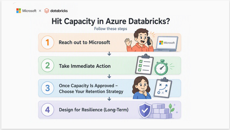
Microsoft's Cloud Architects: Manu Mehta manumehta, Chris Walk cwalk, Eduardo Dos Santos eduardomdossantos, Maria Hito mariahito, Kiran Raja Ch KiranRaja, Paul Singh PaulSingh, Aladdin Alchalabi AladdinAlchalabi and Rafia Aqil Rafia_Aqil Start Here: Engage Microsoft Capacity constraints in Azure Databricks are not an Azure Databricks product issue. Azure Databricks does not own or reserve compute, it dynamically provisions VMs from Azure when clusters are created or scaled. This means cluster creation, autoscaling, or job execution can stall when the underlying VM SKUs are constrained at the regional level. The fastest path to resolution is a structured conversation with your Microsoft account team, who can engage the Azure capacity intake process on your behalf. Create a Quota Support Ticket via Microsoft Support and bring the following to your account team with your Support Ticket Number. Each field maps directly to what capacity intake teams will ask for: missing fields slow the request. What to Prepare Before You Reach Out Your Account Team Field What Capacity Intake Needs Example Subscription IDs The exact Azure subscriptions that will host the workspaces and clusters 7ebee83d-7923-426c-8449-59fd4dff25ab Region(s) Primary region, plus any acceptable alternates East US 2 VM family / SKU Specific series and version requested Eadsv5, ESv4, DSv4, DSv2 Core count / new limit Total vCPU or core count per SKU 10,000 cores for Eadsv5 Workload characteristic CPU-bound vs. memory/shuffle-heavy vs. IO-heavy; batch vs. streaming vs. SQL “Memory-intensive ETL with large joins and shuffles” Scale and timing When you need it, ramp profile, peak vs. steady state “Need by month-end; ramp from 2,000 to 9,650 cores over Q3” Business context Business use case “Migration off AWS” What “Capacity” Really Means: A Layered Mental Model Before diving into fixes, it is important to understand what is actually happening behind the scenes. Capacity constraints can occur at three distinct layers, and solving them requires addressing each one. Layer 1: Azure Infrastructure This is the layer most teams underestimate. Capacity here is governed by: VM SKU availability in the region. D-series and E-series: the two most common Databricks worker families: have repeatedly hit capacity constraints across multiple Azure regions, causing cluster creation failures, autoscale stalls, and provisioning delays. Regional supply constraints, which are dynamic and shared across all Azure tenants. vCPU quotas and limits per subscription, which are separate from regional supply. Quota is your subscription’s limit to deploy resources (like a credit card limit); regional capacity is the underlying infrastructure available. Both must be sufficient. Mechanism Guarantees Capacity Costs Money when idle Discount vCPU quota No No N/A Instance pool Best effort Yes (VM only, no DBU) No Reserved Instance No N/A Yes Savings Plan No N/A Yes CRG Yes, within SLA Yes No, but RI/SP can apply Serverless Platform-Managed No N/A Layer 2: Azure Databricks Platform The Azure Databricks control plane has its own published ceilings that your architecture must proactively respect. Key limits from the official Azure Databricks resource limits documentation: Resource Limit Scope Jobs created per hour 10,000 Workspace Tasks running simultaneously 2,000 Workspace (Run Job and For Each parent tasks excluded) Parent tasks running simultaneously (Run Job / For Each) 750 Workspace SQL warehouses 1,000 Workspace Attached notebooks or execution contexts 145 Cluster Virtual machines 25,000 Per subscription per region Note: For limits marked as non-fixed in the official documentation, you can request an increase through your Azure Databricks account team. Reference: https://learn.microsoft.com/en-us/azure/databricks/resources/limits Layer 3: Workload (Spark Execution) Even when both lower layers cooperate, Spark’s own execution model can produce capacity-like symptoms: Parallelism and task distribution, which dictate how many cores a job can usefully consume. Memory pressure from joins, shuffles, and skewed keys. IO demand and caching behavior, including Delta cache effectiveness and Spark cache misuse. Understanding these layers is critical. Retries sometimes succeed because capacity is dynamic: as other workloads complete, nodes are released back to Azure and briefly become available. Recognizing When You’ve Hit Capacity Capacity issues rarely present as a single clean error. Instead, they appear as inconsistent behaviors: Clusters stuck in Pending state Autoscaling fails or never reaches the desired size Jobs intermittently fail to start Retry attempts sometimes succeed These inconsistencies occur because capacity is shared across Azure tenants and fluctuates throughout the day. Running workloads outside peak business hours in the impacted region’s time zone is one of the most effective short-term mitigations. Inconsistent symptoms are not the same as unknowable ones. Before escalating, confirm what you are actually looking at. Several very different problems produce the symptoms above, and only one of them is a regional capacity shortage. 1. Where to look first Start with the cluster's termination reason and event log in the Azure Databricks workspace. Then cross-check the Azure Activity Log for the workspace's managed resource group over the same time window, which shows the VM allocation attempt and its result. 2. Match signal to the clause What you observe Points to Review What to do Cluster-provider launch or stockout failure Regional capacity for that VM size Immediate Actions, below Quota, core, or vCPU limit referenced Subscription quota, not capacity Request a quota increase — capacity may be fine VM size unavailable in the region or zone Availability restriction, not a transient shortage Switch VM SKU or Family below, retrying will not help Pool returns INSTANCE_POOL_MAX_CAPACITY_FAILURE A Databricks pool ceiling you configured Raise the pool's maximum capacity Cluster starts normally but jobs run slowly, spill, or OOM Workload design, not capacity Why Adding more Nodes is Not Always the Answer, below Only the first row is a genuine Azure capacity constraint. The others are resolved without any capacity conversations 3. Check quota before you conclude capacity Quota and capacity fail in similar ways but are resolved through entirely different paths. Compare current usage against the limit for the VM series and region in question. If usage is below the limit and allocation still fails, the constraint is regional capacity. If usage it at the limit, it is quota and an increase may resolve it outright. Immediate Actions: How to Unblock Your Workloads When you are actively hitting capacity constraints, speed matters. Please reach out to your Microsoft Account team and try these mitigations that are ordered from quickest to most involved. Retry and Run During Off-Peak Hours Capacity availability changes throughout the day as workloads complete and release VMs. Running outside peak business hours for the impacted region significantly improves success rates. Retrying is bounded, not unlimited. As a rule of thumb, retry two or three times across different hours, including at least one off-peak window in the impacted region's time zone. If the same VM size and region fall consistently across a full business day, stop treating it as transient; open a support ticket, engage your account team, and evaluate VM families in parallel. If the workload is production critical with a fixed deadline, or if failures are blocking a migration or cutover already in flight, escalate immediately without waiting for the retry window. Switch VM SKU or Family If a specific VM SKU is constrained, switching to another can immediately unblock provisioning. Move within the same family (for example, DSv4 → DSv5) Or switch families entirely (for example, D-series → F-series or L-series) Choosing the Right VM Family Most Databricks environments default to D-series (general purpose) and E-series (memory optimized). These are also the most heavily used and most capacity-constrained VM families. Consider alternatives based on your workload: VM Family Best For When to Use Trade-off D-series General workloads Default choice Often constrained in high-demand regions E-series Memory-heavy Spark jobs Joins, shuffles, analytics High demand; higher cost F-series CPU-intensive jobs Parsing, transformations Lower memory per core L-series IO-heavy workloads Delta caching, large datasets Higher cost; large local NVMe Practical decision framework: Memory-bound workloads (joins, shuffles): Move from E-series to L-series. Similar memory per core, plus large local NVMe for Delta caching. CPU-bound workloads: Move from D-series to F-series. Higher CPU performance at lower cost. IO-heavy or cache-sensitive workloads: L-series can significantly improve performance and reduce shuffle pressure. Implement Regional Diversity in your Databricks workload As Azure capacity constraints are region and SKU-specific, it is important to build architectural flexibility into your Databricks deployments. For critical or large-scale workloads, consider deploying multiple Databricks workspaces across different Azure regions to reduce dependency on any single region’s capacity. This approach enables: improved resilience to regional capacity constraints greater flexibility in workload placement Important: Multi-region deployment requires deliberate architecture, including deploying separate workspaces and replicating data and configurations across regions; it is not automatic. Why Adding More Nodes Is Not Always the Answer When jobs slow down, the instinct is to scale compute. With Spark, more nodes do not always solve the problem. Common workload issues that masquerade as capacity problems: Data skew Excessive shuffle operations Inefficient partitioning Overuse of UDFs In some workloads, shuffle operations can grow significantly larger than the original input data, placing substantial pressure on compute, memory, disk I/O, and network resources. Because shuffle workloads are distributed across the cluster, adding nodes can improve performance by increasing parallelism. However, that benefit reaches a limit when the bottleneck is caused by data skew, oversized shuffle partitions, network-intensive data movement, or data explosion from joins and aggregations. In these scenarios, the workload becomes constrained by the shuffle pattern itself, and simply adding more nodes does not address the root cause. Instead, the shuffle strategy, partitioning approach, or query design should be optimized. Smarter optimization strategies: Reduce shuffle through repartitioning and query optimization Enable Photon for faster execution Optimize Delta tables using Z-ordering and compaction Leverage caching strategically (not just Spark cache: use the Delta/disk cache) These optimizations can reduce your dependency on scarce VM capacity altogether. Review optimization strategies: The Complete Guide to Azure Databricks Cost Optimization | Microsoft Community Hub. What to Do When Your Capacity Is Approved Once Azure approves your capacity request, retaining it requires active steps. Because Azure capacity is dynamic and shared, approved capacity is held only while compute remains actively deployed and running. This is especially important in highly constrained regions. Microsoft recommends the following: Configure an Instance Pool For workloads that cannot yet use serverless compute, configure an Azure Databricks Instance Pool with a minimum number of idle nodes aligned to your production requirements. An instance pool pre-allocates and maintains a set of idle, ready-to-use VM instances. When a cluster is created from the pool, it draws from these warm nodes: eliminating the need to request new VMs from the regional Azure capacity pool between job runs. Key behaviors: The pool holds a minimum number of nodes continuously, keeping them warm and immediately available. Clusters attached to the pool pull from warm nodes, avoiding re-acquisition from Azure between runs. No DBU charges apply while nodes are idle in the pool. Azure VM infrastructure costs do apply for all minimum idle instances. Size the pool conservatively: aligned to production need only: to balance capacity retention against ongoing cost. Important: Instance pools hold idle nodes on a best-effort basis. Periodic platform events can recycle pool nodes, briefly causing the pool to fall below its configured minimum idle count while Azure re-acquires replacement nodes. Pools significantly improve availability and startup latency, but they do not change the fact that the underlying VMs are still requested from Azure on demand. They are not a hard reservation. Reference: https://learn.microsoft.com/en-us/azure/databricks/compute/pools You can launch a pool's instances against an Azure capacity reservation group by setting the capacity_reservation_group field in the pool's azure_attributes to the group's resource ID. Configure it through the Instance Pools API or the Azure Databricks SDKs. The same requirements apply as for clusters: on-demand instances only, and only workspaces that use VNet injection. Designing for Resilience: Long-Term Best Practices To avoid repeated capacity issues, your architecture needs to evolve beyond reactive mitigations. Plan Ahead with Azure Capacity Reservation Groups For organizations running mission-critical Azure Databricks workloads, Azure Capacity Reservation Groups (CRGs) can provide additional predictability by reserving VM capacity in advance for your Databricks compute resources. Rather than competing for available regional capacity during periods of high demand, reserved capacity helps ensure that the required VM families are available when clusters need to scale or start, Reference: Databricks Clusters API documentation. Note: Before you commit to a reservation, know three things: Auto-termination stops saving VM costs. When a cluster terminates, its reserved capacity returns to an unused state and continues billing at the full VM rate. A pool backed by a reservation is not billed twice. If a team already pays for minimum idle pool nodes in a constrained region, a reservation at comparable spend converts best-effort capacity into SLA-backed capacity. Confirm that the cluster is actually using the reservation. Creating the reservation proves Azure set capacity aside, but it does not prove Databricks is drawing on it. Start a cluster, then check that allocated instances on the reservation rose by the expected node count. If it stays at zero, the usual causes are a VM size mismatch, availability not set to ON_DEMAND_AZURE, a workspace on the Databricks-managed VNet, or the RBAC actions never granted. Note also that omitting capacity_reservation_group when editing an instance pool silently clears it. Step-by-Step Instructions: Attaching a CRG to Databricks is done only through the Clusters/Instance Pools API or the Databricks SDKs, it is not available in the compute UI. Prerequisites VNet-injected workspace only. The workspace must be deployed into your own VNet. Workspaces on the default Databricks-managed VNet cannot use a CRG. On-demand instances only. The cluster/pool must use ON_DEMAND_AZURE availability. Spot and serverless are not eligible. Same region. Create the CRG in the same Azure region as the workspace. Matching VM size. Reserve the exact VM SKU(s) your cluster uses (driver and workers). Sufficient subscription quota for that SKU and core count. Go to the CRG resource -> Access Control -> Add role assignment and add the below roles to the workspace (i.e. databricks-login-prod) Enterprise Application: Microsoft.Compute/capacityReservationGroups/read Microsoft.Compute/capacityReservationGroups/deploy/action Microsoft.Compute/capacityReservationGroups/capacityReservations/read Microsoft.Compute/capacityReservationGroups/capacityReservations/deploy/action Step 1: Create the CRG and reservation in Azure az group create -l eastus -g myResourceGroup az capacity reservation group create \ -n myCapacityReservationGroup -l eastus -g myResourceGroup --zones 1 2 3 az capacity reservation create \ -c myCapacityReservationGroup -n myCapacityReservation \ -l eastus -g myResourceGroup --sku Standard_D2s_v3 --capacity 5 --zone 1 Note: If you want to create the CRG from the Azure Portal you can do the following: Set Subscription, Resource group, Name, and Region (use the same region as your Databricks workspace). Optionally pick Availability zones. Add one or more reservations: Reservation name, Instances (quantity), and VM size (match your cluster's driver/worker SKU). Example here: reservation-eadsv5, 5 × Standard_D4s_v3. Confirm the summary (price, basics, reservations), then click Create. Step 2 Attach the CRG to the cluster (Clusters API or SDK) This would be the Azure Databricks compute cluster, the Spark cluster you create inside your Azure Databricks workspace (Compute → Create compute, or a job cluster). You add an azure_attributes block to the cluster definition. The snippet below is a fragment that goes inside the cluster's JSON, alongside the normal cluster fields. You provide the CRG resource ID; Azure picks a matching reservation within the group. databricks clusters edit --json '{ "cluster_id": "<existing-cluster-id>", "spark_version": "15.4.x-scala2.12", "node_type_id": "Standard_D4s_v3", "num_workers": 4, "azure_attributes": { "availability": "ON_DEMAND_AZURE", "capacity_reservation_group": "/subscriptions/<subscription-id>/resourceGroups/<resource-group>/providers/Microsoft.Compute/capacityReservationGroups/<crg-name>" } }' The cluster's node_type_id (VM SKU) has to be the same VM size you reserved in the CRG (Step 1). If the reservation is Standard_D4s_v3, the cluster's node type must also be Standard_D4s_v3, or it won't draw from the reservation. For instance pools, set the same capacity_reservation_group field via the Instance Pools API or SDK (If you omit the field when editing a pool, Databricks clears any CRG already configured on it). Plan for Capacity Early Understand VM quotas and limits before you need them: not after a constraint occurs. Avoid designing a single SKU. Build flexibility into cluster configurations so you can switch families without re-engineering jobs. Standardize Compute Configurations Consistent, policy-driven environments make it easier to adapt when capacity constraints occur. Use Databricks Cluster Policies to constrain cluster creation to approved, available VM families: this prevents teams from inadvertently requesting constrained SKUs. Also, consider enforcing the CRG setting through a Databricks compute policy, so teams launch only against approved, reserved capacity. Move Toward Serverless Where Possible Serverless compute abstracts capacity management away from the customer. As the Databricks platform expands serverless support, migrating eligible workloads is the most durable long-term strategy. Azure continues to expand infrastructure capacity, but there are no guaranteed timelines for relief in constrained regions. Note: If your workload supports serverless compute, Databricks recommends using serverless compute instead of pools or classic VM-backed clusters. Serverless removes dependency on specific VM SKUs and regional capacity: scaling is managed by the platform with significantly improved availability. Reference: https://learn.microsoft.com/en-us/azure/databricks/serverless-compute. For eligible workloads: including Databricks Jobs (automated workflows), Databricks SQL Warehouses, and Delta Live Tables: serverless compute eliminates VM SKU dependency entirely. Configuration guidance is available in the Azure Databricks deployment guide, Development Section, Step 9. Multi-Region Strategy for Critical Workloads For the most critical workloads, evaluate a multi-region deployment as part of your business's continuity planning. This is a significant architectural investment: see the FAQ for the full scope: but it is the only approach that provides true regional redundancy. Coordinate this with your Microsoft account team. Reference: Azure Databricks & Microsoft Fabric Disaster Recovery: The Complete Better‑Together Strategy for Cloud Architects Know the Difference: Azure Capacity Reservations vs. Reserved Instances vs. Savings Plans When planning Azure infrastructure, it is important to separate capacity assurance from cost optimization. Although these options are sometimes discussed together, they solve different problems. On-Demand Capacity Reservations (ODCR) are designed to reserve compute capacity for workloads that need to run now. They are useful when an organization needs capacity for an eligible VM size in a specific region or availability zone. ODCRs generally offer flexibility because they do not require a long-term commitment and can be canceled when no longer needed. Future Capacity Reservations (FCR) support planned capacity requirements for a future need-by date. They are useful for migrations, major launches, seasonal events, and other predictable workload ramps that require advance capacity planning. In comparison, Azure Reserved VM Instances and Azure Savings Plans for Compute are primarily commercial constructs. Reserved Instances provide discounts for predictable, consistently running workloads through a one-year or three-year commitment. Savings Plans offer broader flexibility by applying discounts to eligible compute usage in exchange for an hourly spending commitment. The key takeaway is simple: capacity reservations address infrastructure availability, while Reserved Instances and Savings Plans address pricing. Organizations can use them together, pairing a capacity reservation with an applicable pricing benefit to improve both workload readiness and cost efficiency. Final Takeaways Capacity issues are infrastructure-level constraints, not Databricks product failures VM family selection is critical: do not rely solely on D-series and E-series Workload optimization can reduce dependency on scarce resources before requesting more capacity Serverless compute is Microsoft’s preferred long-term recommendation for eligible workloads Architectural flexibility: multi-SKU, multi-region awareness is your best defense against future constraints FAQ Why do retries work? Capacity in Azure regions is shared across all tenants and fluctuates throughout the day as workloads complete and release VMs. A retry succeeds when capacity temporarily frees up. Retrying during off-peak hours improves success rates significantly. Why does capacity fluctuate during the day? Capacity is a function of regional supply and concurrent demand. As workloads complete, nodes are released back to Azure. Peak business hours in the impacted region’s time zone tend to be the tightest windows. Why are instance pools not a hard reservation? Pools hold a minimum number of nodes on a best-effort basis. Periodic platform events recycle pool nodes, so a pool can briefly fall below its configured minimum idle count while Azure re-acquires replacement nodes. Setting minimum idle to 0 avoids paying for idle VMs at the cost of slower acquisition time. Pools significantly improve availability and startup latency but do not guarantee capacity at the Azure infrastructure level. Why does serverless behave differently from classic clusters? Serverless compute removes customer control over individual VM SKUs. Databricks manages the underlying capacity across a shared pool. SKU-swap and pool-based mitigations do not apply. Customer-side levers reduce to retry and off-peak scheduling. The trade-off is that serverless is the simplest and most reliable option when the workload supports it. Why is changing regions a last resort? Region changes require redeployment of the Azure Databricks workspace and migration of all dependent artifacts: jobs, clusters, libraries, networking (private endpoints, VNet injection), Unity Catalog assignments, identities, and source data. The destination region must be validated for the same SKU and zonal configuration. For these reasons, region change should always be coordinated with the Microsoft account team and attempted only after preferred mitigations have been exhausted. Why does VM family selection matter so much for capacity? Different VM families have different supply curves. D-series and E-series are the most requested Databricks worker families and the ones most frequently constrained. Choosing a SKU based on whether the workload is memory/shuffle-heavy, CPU-bound, or IO-heavy improves both performance and the probability that capacity is available. The capacity team often steers customers toward newer-generation alternatives when supply differs by generation version. What does the Microsoft account team actually do? They route the request into the Azure capacity intake process, advise alternate SKUs and regions, surface zonal vs. regional considerations, and provide forward visibility into known constraints. The customer’s job is to bring a complete, accurate workload profile so the account team can advocate effectively. It is also recommended to open an Azure Support ticket. This will save time later, as the capacity planning teams would like to track issues and requests via a support ticket. Once an Azure Support ticket is opened, the ticket number should be shared to the Microsoft Account Team, at a minimum to the Customer Success Account Manager (CSAM), if one is assigned to your organization.725Views1like0CommentsComplete Guide to Azure Databricks Cost Optimization for Data Engineers
Co-Authored by: Aladdin Alchalabi AladdinAlchalabi, Sanjeev Nair Sanjeev Nair and Rafia Aqil Rafia_Aqil This guide walks through a proven approach to Azure Databricks cost optimization, structured in three phases: 1. Discovery, 2. Cluster/Data/Code Best Practices, and 3. Team Alignment & Next Steps. Phase 1: Discovery Assessing Your Current State The following questions are designed to guide your initial assessment and help you identify areas for improvement. Documenting answers to each will provide a baseline for optimization and inform the next phases of your cost management strategy. Environment & Organization Cluster Management Cost Optimization Data Management Performance Monitoring Future Planning What is the current scale of your Databricks environment? How many workspaces do you have? How are your workspaces organized (e.g., by environment type, region, use case)? How many clusters are deployed? How many users are active? What are the primary use cases for Databricks in your organization? Data engineering Data science Machine learning Business intelligence How are clusters currently managed? Manual configuration Automated scripts Databricks REST API Cluster policies What is the average cluster uptime? Hours per day Days per week What is the average cluster utilization rate? CPU usage Memory usage What is the current monthly spend on Databricks? Total cost Breakdown by workspace Breakdown by cluster What cost management tools are currently in use? Azure Cost Management Third-party tools Are there any existing cost optimization strategies in place? Reserved instances Spot instances Cluster auto-scaling What is the current data storage strategy? Data lake Data warehouse Hybrid What is the average data ingestion rate? GB per day Number of files What is the average data processing time? ETL jobs Machine learning models What types of data formats are used in your environment? Delta Lake Parquet JSON CSV Other formats relevant to your workloads What performance monitoring tools are currently in use? Databricks Ganglia Azure Monitor Third-party tools What are the key performance metrics tracked? Job execution time Cluster performance Data processing speed Are there any planned expansions or changes to the Databricks environment? New use cases Increased data volume Additional users What are the long-term goals for Databricks cost optimization? Reducing overall spend Improving resource utilization & cost attribution Enhancing performance Understanding Databricks Cost Structure Total Cost = Cloud Cost + DBU Cost Cloud Cost: Compute (VMs, networking, IP addresses), storage (ADLS, MLflow artifacts), other services (firewalls), cluster type (serverless compute, classic compute) DBU Cost: Workload size, cluster/warehouse size, photon acceleration, compute runtime, workspace tier, SKU type (Jobs, Delta Live Tables, All Purpose Clusters, Serverless), model serving, queries per second, model execution time Diagnose Cost and Issues Effectively diagnosing cost and performance issues in Databricks requires a structured approach. Use the following steps and metrics to gain visibility into your environment and uncover actionable insights. 1. Identify Costly Workloads Account Console Usage Reports: Review usage reports to identify usage breakdowns by product, SKU name, and custom tags. Usage Breakdown by Product and SKU: Helps you understand which services and compute types (clusters, SQL warehouses, serverless options) are consuming the most resources. Custom Tags for Attribution: Tags allow you to attribute costs to teams, projects, or departments, making it easier to identify high-cost areas. Workflow and Job Analysis: By correlating usage data with workflows and jobs, you can pinpoint long-running or resource-heavy workloads that drive costs. Focus on Long-Running Workloads: Examine workloads with extended runtimes or high resource utilization. Key Question: Which pipelines or workloads are driving the majority of your costs? Governance Hub: is a centralized, account-level UI for monitoring and managing governance across Databricks. Note this is a beta feature, we will update this article as we get more information and use-cases on this feature. Now That You’ve Identified Long-Running Workloads, Review These Key Areas: 2. Review Cluster Metrics CPU Utilization: Track guest, iowait, idle, irq, nice, softirq, steal, system, and user times to understand how compute resources are being used. Memory Utilization: Monitor used, free, buffer, and cached memory to identify over- or under-utilization. Key Question: Is your cluster over- or under-utilized? Are resources being wasted or stretched too thin? 3. Review SQL Warehouse Metrics Live Statistics: Monitor warehouse status, running/queued queries, and current cluster count. Time Scale Filter: Analyze query and cluster activity over different time frames (8 hours, 24 hours, 7 days, 14 days). Peak Query Count Chart: Identify periods of high concurrency. Completed Query Count Chart: Track throughput and query success/failure rates. Running Clusters Chart: Observe cluster allocation and recycling events. Query History Table: Filter and analyze queries by user, duration, status, and statement type. Key Question: Is your SQL Warehouse over- or under-utilized? Are resources being wasted or stretched too thin? 4. Review Spark UI Stages Tab: Look for skewed data, high input/output, and shuffle times. Uneven task durations may indicate data skew or inefficient data handling. Jobs Timeline: Identify long-running jobs or stages that consume excessive resources. Stage Analysis: Determine if stages are I/O bound or suffering from data skew/spill. Executor Metrics: Monitor memory usage, CPU utilization, and disk I/O. Frequent garbage collection or high memory usage may signal the need for better resource allocation. 4.1. Spark UI: Storage & Jobs Tab Storage Level: Check if data is stored in memory, on disk, or both. Size: Assess the size of cached data. Job Analysis: Investigate jobs that dominate the timeline or have unusually long durations. Look for gaps caused by complex execution plans, non-Spark code, driver overload, or cluster malfunction. 4.2. Spark UI: Executor Tab Storage Memory: Compare used vs. available memory. Task Time (Garbage Collection): Review long tasks and garbage collection times. Shuffle Read/Write: Measure data transferred between stages. 5. Additional Diagnostic Methods System Tables in Unity Catalog: Query system tables for cost attribution and resource usage trends. Cost Observability Queries Tagging Analysis: Use tags to identify which teams or projects consume the most resources. Dashboards & Alerts: Set up cost dashboards and budget alerts for proactive monitoring. Phase 2: Cluster/Code/Data Best Practices Alignment Cluster UI Configuration and Cost Attribution Effectively configuring clusters/workloads in Databricks is essential for balancing performance, scalability, and cost. Tunning settings and features when used strategically can help organizations maximize resource efficiency and minimize unnecessary spending. Key Configuration Strategies 1. Reduce Idle Time: Clusters to incur costs even when not actively processing workloads. To avoid paying for unused resources: Enable Auto-Terminate: Set clusters automatically shut down after a period of inactivity. This simple setting can significantly reduce wasted spending. Enable Autoscaling: Workloads fluctuate in size and complexity. Autoscaling allows clusters to dynamically adjust the number of nodes based on demand: Automatic Resource Adjustment: Scale up for heavy jobs and scale down for lighter loads, ensuring you only pay for what you use. It significantly enhances cost efficiency and overall performance. For serverless and streaming, using Delta Live Tables with autoscaling is recommended. This approach leads to better resource management and reliability. Use Spot Instances: For batch processing and non-critical workloads, spot instances offer substantial cost savings: Lower VM Costs: Spot instances are typically much cheaper than standard VMs. However, they are not recommended for jobs requiring constant uptime due to potential interruptions. Considerations: Azure Spot VMs are intended for non-critical, fault-tolerant tasks. They can be evicted without notice, risking production stability. No SLA guarantees mean potential downtime for critical applications. Using Spot VMs could lead to reliability issues in production environments. Leverage Photon Engine: Photon is Databricks’ high-performance, vectorized query engine: Accelerate Large Workloads: Photon can dramatically reduce runtime for compute-intensive tasks, improving both speed and cost efficiency. Keep Runtimes Up to Date: Using the latest Databricks runtime ensures optimal performance and security: Benefit from Improvements: Regular updates include performance enhancements, bug fixes, and new features. Apply Cluster Policies: Cluster policies help standardize configurations and enforce cost controls across teams: Governance and Consistency: Policies can restrict certain settings, enforce tagging, and ensure clusters are created with cost-effective defaults. Optimize Storage: type impacts both performance and cost: Switch from HDDs to SSDs: SSDs provide faster caching and shuffle operations, which can improve job efficiency and reduce runtime. Tag Clusters for Cost Attribution: Tagging clusters enables granular tracking and reporting: Visibility and Accountability: Use tags to attribute costs to specific teams, projects, or environments, supporting better budgeting and chargeback processes. Select the Right Cluster Type: Different workloads require different cluster types, see table below for Serverless vs Classic Compute: Feature Classic Compute Serverless Compute Control Full control over config & network Minimal control, fully managed by Databricks Startup Time Slower (unless pre-warmed) Instant Cost Model Hourly, supports reservations Pay-per-use, elastic scaling Security VNet injection, private endpoints NCC-based private connectivity Best For Heavy ETL, ML, compliance workloads Interactive queries, unpredictable demand Job Clusters: Ideal for scheduled jobs and Delta Live Tables. All-Purpose Clusters: Suited for ad-hoc analysis and collaborative work. Single-Node Clusters: Efficient for simple exploratory data analysis or pure Python tasks. Serverless Compute: Scalable, managed workloads with automatic resource management. 11. Monitor and Adjust Regularly: review cluster metrics and query history: Continuous Optimization: Use built-in dashboards to monitor usage, identify bottlenecks, and adjust cluster size or configuration as needed. Code Best Practices Avoid Reprocessing Large Tables Use a CDC (Change Data Capture) architecture with Delta Live Tables (DLT) to process only new or changed data, minimizing unnecessary computation. Ensure Code Parallelizes Well Write Spark code that leverages parallel processing. Avoid loops, deeply nested structures, and inefficient user-defined functions (UDFs) that can hinder scalability. Reduce Memory Consumption Tweak Spark configurations to minimize memory overhead. Clean out legacy or unnecessary settings that may have carried over from previous Spark versions. Prefer SQL Over Complex Python Use SQL (declarative language) for Spark jobs whenever possible. SQL queries are typically more efficient and easier to optimize than complex Python logic. Modularize Notebooks Use %run to split large notebooks into smaller, reusable modules. This improves maintainability. Use LIMIT in Exploratory Queries When exploring data, always use the LIMIT clause to avoid scanning large datasets unnecessarily. Monitor Job Performance Regularly review Spark UI to detect inefficiencies such as high shuffle, input, or output. Review the below table for optimization opportunities: Spark stage high I/O - Azure Databricks | Microsoft Learn Databricks Code Performance Enhancements & Data Engineering Best Practices By enabling the below features and applying best practices, you can significantly lower costs, accelerate job execution, and build Databricks pipelines that are both scalable and highly reliable. For more guidance review: Comprehensive Guide to Optimize Data Workloads | Databricks. Feature / Technique Purpose / Benefit How to Use / Enable / Key Notes Disk Caching Accelerates repeated reads of Parquet files Set spark.databricks.io.cache.enabled = true Dynamic File Pruning (DFP) Skips irrelevant data files during queries, improves query performance Enabled by default in Databricks Low Shuffle Merge Reduces data rewriting during MERGE operations, less need to recalculate ZORDER Use Databricks runtime with feature enabled Adaptive Query Execution (AQE) Dynamically optimizes query plans based on runtime statistics Available in Spark 3.0+, enabled by default Deletion Vectors Efficient row removal/change without rewriting entire Parquet file Enable in workspace settings, use with Delta Lake Materialized Views Faster BI queries, reduced compute for frequently accessed data Create in Databricks SQL Optimize Compacts Delta Lake files, improves query performance Run regularly, combine with ZORDER on high-cardinality columns ZORDER Physically sorts/co-locates data by chosen columns for faster queries Use with OPTIMIZE, select columns frequently used in filters/joins Auto Optimize Automatically compacts small files during writes Enable optimizeWrite and autoCompact table properties Liquid Clustering Simplifies data layout, replaces partitioning/ZORDER, flexible clustering keys Recommended for new Delta tables, enables easy redefinition of clustering keys File Size Tuning Achieve optimal file size for performance and cost Set delta.targetFileSize table property Broadcast Hash Join Optimizes joins by broadcasting smaller tables Adjust spark.sql.autoBroadcastJoinThreshold and spark.databricks.adaptive.autoBroadcastJoinThreshold Shuffle Hash Join Faster join alternative to sort-merge join Prefer over sort-merge join when broadcasting isn’t possible, Photon engine can help Cost-Based Optimizer (CBO) Improves query plans for complex joins Enabled by default, collect column/table statistics with ANALYZE TABLE Data Spilling & Skew Handles uneven data distribution and excessive shuffle Use AQE, set spark.sql.shuffle.partitions=auto, optimize partitioning Data Explosion Management Controls partition sizes after transformations (e.g., explode, join) Adjust spark.sql.files.maxPartitionBytes, use repartition() after reads Delta Merge Efficient upserts and CDC (Change Data Capture) Use MERGE operation in Delta Lake, combine with CDC architecture Data Purging (Vacuum) Removes stale data files, maintains storage efficiency Run VACUUM regularly based on transaction frequency Phase 3: Team Alignment and Next Steps Implementing Cost Observability and Taking Action Effective cost management in Databricks goes beyond configuration and code—it requires robust observability, granular tracking, and proactive measures. Below outlines how your teams can achieve this using system tables, tagging, dashboards, and actionable scripts. Cost Observability with System Tables Databricks Unity Catalog provides system tables that store operational data for your account. These tables enable historical cost observability and empower FinOps teams to analyze spend independently. System Tables Location: Found inside the Unity Catalog under the “system” schema. Key Benefits: Structured data for querying, historical analysis, and cost attribution. Action: Assign permissions to FinOps teams so they can access and analyze dedicated cost tables. Enable Tags for Granular Tracking Tagging is a powerful feature for tracking, reporting, and budgeting at a granular level. Classic Compute: Manually add key/value pairs when creating clusters, jobs, SQL Warehouses, or Model Serving endpoints. Use cluster policies to enforce custom tags. Serverless Compute: Create budget policies and assign permissions to teams or members for serverless workloads. Action: Tag all compute resources to enable detailed cost attribution and reporting. Track Costs with Dashboards and Alerts Databricks offers prebuilt dashboards and queries for cost forecasting and usage analysis. Dashboards: Visualize spend, usage trends, and forecast future costs. Prebuilt Queries: Use top queries with system tables to answer meaningful cost questions. Budget Alerts: Set up alerts in the Account Console (Usage > Budget) to receive notifications when spend approaches defined thresholds. Build Culture of Efficiency To go beyond technical fixes and build a culture of efficiency, by focusing on the below strategic actions: Collaborate with Internal Engineers: Spend time with engineering teams to understand workload patterns and optimization opportunities. Peer Reviews and Code Audits: Conduct regular code review sessions and peer reviews to ensure best practices are followed for Spark jobs, data pipelines, and cluster configurations. Create Internal Best Practice Documentation: Develop clear guidelines for writing optimized code, managing data, and maintaining clusters. Make these resources easily accessible for all teams. Implement Observability Dashboards: Use Databricks’ built-in features to create dashboards that track spend, monitor resource utilization, and highlight anomalies. Set Alerts and Budgets: Configure alerts for long-running workloads and establish budgets using prebuilt Databricks capabilities to prevent cost overruns. 5. Azure Reservations and Azure Savings Plan When optimizing Databricks costs on Azure, it’s important to understand the two main commitment-based savings options: Azure Reservations and Azure Savings Plans. Both can help you reduce compute costs, but they differ in flexibility and how savings are applied. Which Should You Choose? Reservations are ideal if you have stable, predictable Databricks workloads and want maximum savings. Savings Plans are better if you expect your compute needs to change, or if you want a simpler, more flexible way to save across multiple services. Pro Tip: You can combine both options—use Reservations for your baseline, always-on Databricks clusters, and Savings Plans for bursty, variable, or new workloads. Summary Table: Action Steps It’s critical to monitor costs continuously and align your teams with established best practices, while scheduling regular code review sessions to ensure efficiency and consistency. Area Best Practice / Action System Tables Use for historical cost analysis and attribution Tagging Apply to all compute resources for granular tracking Dashboards Visualize spend, usage, and forecasts Alerts Set budget alerts for proactive cost management Scripts/Queries Build custom analysis tools for deep insights Cluster/Data/Code Review & Align Regularly review best practices, share findings, and align teams on optimization Save on your Usage Consider Azure Reservations and Azure Savings Plan905Views2likes0CommentsEnabling the Compliance Security Profile (CSP) for HIPAA on Azure Databricks
Microsoft Architect's: Aladdin Alchalabi AladdinAlchalabi, Kiran Raja KiranRaja, Peter Lenges PeterLenges, Jessica Reece jareece, Benjamin Coughtry bcoughtry, Anishek Kamal anishekkamal, Tayo Akigbogun takigbogun, Eric Kwashie ekwashie, Peter Lo PeterLo and Rafia Aqil Rafia_Aqil Peer Reviewed: Ted Kim tedkim and Arvind Periyasamy ArvindPeriyasamy Purpose and WHY Azure Databricks has put in place controls to meet the unique compliance needs of highly regulated industries. The requirement for the compliance security profile (CSP) is a joint effort between Microsoft and Databricks for Azure-Databricks workspaces. The value proposition of the compliance security profile is that it provides Customers significantly more hardening and security features. Mandatory Deadline: The Compliance Security Profile (CSP) becomes mandatory for processing HIPAA, HITRUST, and IRAP regulated data on Azure-Databricks by September 1, 2026. Key Dates: Enable the Compliance Security Profile and select HIPAA by September 1, 2026. Prepare for Azure Virtual Network encryption enforcement beginning February 1, 2027. Compliance Responsibility: Enabling CSP supports applicable technical controls but does not, by itself, establish HIPAA compliance. Compliance is a shared responsibility among the customer, Microsoft, and Databricks. Customers must evaluate their administrative, physical, and technical safeguards and confirm that an applicable Microsoft Business Associate Agreement is in place. Enabling CSP on Workspaces These requirements are checked and enforced on new workspaces today, with enforcement on existing workspaces expected in the future; where prerequisites are missing, clusters may fail to start. Prerequisite Requirement Costs There is a 10% cost of the Azure Databricks product spend within each workspace where CSP is enabled. **Review with your account team for any grace period during which the Enhanced Security & Compliance (ESC) add-on is available at no charge. After the grace period ends, a 10% DBU upcharge applies. Enhanced Security & Compliance add-on For existing workspaces: From Azure portal, click the Settings > Security & compliance on an existing Azure Databricks workspace: **Review Note #2 below Azure VNet encryption Azure Virtual Network encryption must be enabled on the Azure Databricks workspace VNet. Infrastructure as code: Update the encryption block on your VNet resource. In Terraform, that's azurerm_virtual_network. Azure portal: Toggle encryption on the VNet (Overview → Properties → Encryption). Command line: Enable it with the Azure CLI or PowerShell. **Review Note #4 below Supported VM instance types Use a VM series that supports VNet encryption and verify compatibility before enabling the profile. **This does not apply to serverless compute. NOTE: Confirm your workspace is using Premium Pricing tier. The profile can be enabled when a workspace is created or on an existing workspace, through the Azure portal, the Azure CLI, PowerShell, an ARM template, or Terraform. Only the Public Preview, Private Preview, and Beta features listed in this section are supported for workspaces with the compliance security profile enabled: Compliance security profile - Azure Databricks | Microsoft Learn Currently, the compliance security profile checks and enforces only the use of specific VM instance types, not the enablement of Azure Virtual Network encryption. Enforcement of the Azure Virtual Network encryption requirement begins on February 1, 2027, including on workspaces that already have the compliance security profile enabled. This flexibility shall allow customers more time to set up VNET encryption. This has been updated in documentation today (See ‘Important’ box). Regarding rollback, CSP can be reversed via a support ticket, if no regulated data has been processed on a particular workspace. Plan for possible effects on cluster startup, networking, feature availability, maintenance operations, and cost. A closer look at VNet encryption CSP is enabled per Databricks workspace, but VNet encryption is applied at the VNet level. Enabling it for a Databricks workload therefore affects every resource within that VNet, not just the workspace. A common approach in a hub-and-spoke design is to leave the hub VNet unencrypted and encrypt only the spoke VNet. The hub typically holds shared services such as the DNS resolver, while the spoke hosts the Databricks workspaces that require CSP. What does it mean for a VNet to be encrypted? An encrypted VNet is a security measure that protects VM-to-VM traffic. Data is encrypted in transit through a DTLS tunnel. This is platform-level encryption, applied automatically to traffic within your VNet and across peered VNets. It requires no changes to your operating system or applications. What happens to my VM-to-VM traffic? Qualifying VM-to-VM traffic is encrypted. Traffic involving unqualified instances simply keeps flowing unencrypted. The only enforcement available today is AllowUnencrypted. Important clarifications Encrypting the VNet does not guarantee all traffic within it will be encrypted. The only traffic that gets encrypted is VM-to-VM traffic where both the source and destination VMs are (1) on a supported SKU and (2) have Accelerated Networking enabled on the network interface. Encrypting the VNet does not drop or break traffic from unsupported SKUs. The only supported GA setting today is to allow unencrypted traffic, so non-qualifying traffic is still permitted; it just isn't encrypted. A future DropUnencrypted setting will drop that traffic instead for further hardening. It isn't available yet, and it's currently unknown whether it will become a required setting for CSP. Review the following recommended steps The steps below represent a validated implementation pattern. The exact network design can vary by environment, but the same prerequisite, isolation, and end-to-end validation principles should be applied. Validated implementation step Recommended approach and expected outcome Isolated sandbox workspace Enable CSP first in a representative non-production workspace. This avoids irreversible changes to DEV or production while the network topology, dependencies, VM compatibility, and operational behavior are validated. Enable CSP and select HIPAA Enable the Compliance Security Profile and select HIPAA under Settings > Security & compliance before processing PHI after September 1, 2026. Enable VNet encryption Enable VNet encryption. **Review Azure Virtual Network encryption limitations: What is Azure Virtual Network encryption? - Azure Virtual Network | Microsoft Learn Start a classic cluster Confirm that a classic cluster starts successfully after CSP and VNet encryption prerequisites are applied. This validates that the selected compute path and VM types remain operational. Validate storage connectivity Confirm storage connectivity continue to work. Confirm rollout readiness Proceed to DEV and production only after the complete private connectivity path, cluster startup, storage access, DNS resolution, data pipelines, and performance have been validated from end to end. Things to Review Enablement is permanent Enabling the compliance security profile, or adding a compliance standard, is intended to be a permanent change. You cannot remove the profile or an individual standard from a workspace that has ever processed regulated data; to revert, you must delete the workspace and create a new one. Validate the configuration in an isolated, representative non-production workspace before enabling DEV or production. Inventory and Assessment Identify Regulated Workspaces: Catalogue all existing Azure-Databricks workspaces. Determine which ones currently process, or are planned to process, data subject to HIPAA, HITRUST, or IRAP. Review Data Pipelines: Map out all data ingress and egress points for these identified workspaces, including connections to on-premises data sources, other cloud services, and external APIs. This helps identify potential network impacts. Verify Prerequisites Before Rollout: Confirm that selected VM instance types support VNet encryption and that every required CSP and networking setting is in place, because missing prerequisites can prevent clusters from starting. Enablement Method: Choose the appropriate tooling for enablement of Azure Portal, Azure CLI, PowerShell, ARM templates, or Terraform to ensure consistency and automation. Keep sensitive data out of customer-defined fields You are solely responsible for ensuring that PHI or other sensitive information is never entered into customer-defined input fields. These include workspace names, compute and resource names, tags, job names, job run names, network names, credential names, storage account names, and Git repository IDs or URLs, all of which may be stored, processed, or accessed outside the compliance boundary. What Changes After Enabling Compliance Security Profile On CSP-enabled workspaces, Partner-powered AI features are disabled by default and some assistive features such as Genie Code are also disabled; a workspace admin can re-enable them if required. In addition, only the specific preview features listed in the compliance security profile documentation are supported. No other Public Preview, Private Preview, or Beta feature may be used to process regulated data. Compliance Security Profile (CSP) enhances the security posture of Azure Databricks by enabling a hardened compute image, enhanced security monitoring, and automatic cluster updates. With automatic cluster updates enabled, classic compute resources are periodically updated and may restart during configured maintenance windows, so production schedules should be planned accordingly. Enhanced security monitoring deploys security monitoring agents on supported compute resources and generates logs that security teams can ingest and analyze. When deploying through ARM templates, CSP, enhancedSecurityMonitoring, and automaticClusterUpdate are configurable security and compliance settings that can be specified as part of the workspace deployment. Why GPU-accelerated compute may be affected Azure Databricks supports several GPU families, but Azure VNet encryption currently documents a narrower GPU list. Please review the list here: What is Azure Virtual Network encryption? - Azure Virtual Network | Microsoft Learn What happens if a customer does not enable Azure Databricks CSP? Azure Databricks has implemented additional controls to support the security and compliance requirements of highly regulated industries. CSP should not be characterized solely as a Microsoft initiative; it is part of the Azure Databricks security and compliance offering delivered by Microsoft and Databricks. CSP provides additional platform hardening and security capabilities, including a CIS Level 1 hardened compute image, automatic cluster updates, enhanced security monitoring, and TLS 1.2 or higher for relevant communications. Beginning September 1, 2026, CSP is required for Azure Databricks workspaces processing data subject to applicable standards, including HIPAA, HITRUST, and IRAP. If a customer chooses not to enable CSP while processing data subject to one of these standards, the workspace would not meet the documented Azure Databricks configuration requirements for that regulated workload. This does not, by itself, determine the customer's overall legal or regulatory compliance; customers should assess their obligations with their legal, compliance, and audit teams. References Compliance security profile: https://learn.microsoft.com/en-us/azure/databricks/security/privacy/security-profile Configure enhanced security and compliance settings: https://learn.microsoft.com/en-us/azure/databricks/security/privacy/enhanced-security-compliance HIPAA, Azure Databricks, Microsoft Learn: https://learn.microsoft.com/en-us/azure/databricks/security/privacy/hipaa What is Azure Virtual Network encryption: https://learn.microsoft.com/en-us/azure/virtual-network/virtual-network-encryption-overview Create a Virtual Network with encryption: https://learn.microsoft.com/en-us/azure/virtual-network/how-to-create-encryption?tabs Hashicorp azurerm_virtual_network: azurerm_virtual_network | Resources | hashicorp/azurerm | Terraform | Terraform Registry2KViews2likes0CommentsMeet the IQ's: How Microsoft is Creating Context-Aware AI
Microsoft Architect's: Allison Rose allisonrose, Lavanya Sreedhar LavanyaSreedhar, Tom Dinh Tom-Dinh, Oviya Soundararajan oviyasound and Rafia Aqil Rafia_Aqil The AI era demands more than powerful language models. It demands context a deep understanding of what enterprise data means, how it connects, and how AI systems can reason and act on it intelligently. Microsoft has been building the foundational intelligence layer that makes this possible: a family of capabilities collectively known as the IQ Platform. The Microsoft IQ Platform is not a single product but a set of complementary intelligence layers: Work IQ, Fabric IQ, Foundry IQ and Web IQ each designed to inject rich contextual understanding into a different part of the enterprise technology stack. Together, they represent Microsoft’s strategic vision for how AI can move beyond isolated answers and become a true operating system for organizational intelligence. This article unpacks each IQ, explains the problems they solve, and explores how they work together to power the next generation of AI-driven enterprise workflows. How the IQs Work Together? Work IQ, Fabric IQ, Foundry IQ, and Web IQ are not competing products or overlapping investments. They are complementary intelligence layers designed to operate across different contexts within the enterprise, and they are most powerful when combined. Work IQ brings the intelligence of Microsoft 365 to every agent and Copilot experience- connecting people, conversations, documents, and organizational signals into a semantic layer that understands how work happens. Fabric IQ brings the intelligence of enterprise data and business context- teaching AI not just what the data says, but what it means in the language of your business: entities, relationships, rules, and governed actions. Foundry IQ brings the infrastructure intelligence that enables all of this to scale- eliminating the undifferentiated plumbing of agentic AI and letting teams focus on building the workflows that actually differentiate their business. Web IQ brings fresh, external web context, helping agents consider current and relevant public information alongside the knowledge and business context inside the organization. Microsoft Web IQ grounds most of the top AI platforms, including Copilot and ChatGPT. Together, the IQ platform represents Microsoft’s answer to one of the defining challenges of the AI era: not just making AI more capable, but making AI contextually aware-grounded in the real knowledge, relationships, and intent of your organization. Fabric IQ: Teaching AI the Language of Business Microsoft Fabric is an end-to-end, unified data analytics platform centered on OneLake- a centralized data lake that stores all analytical and operational business data in open Delta format. Because every Fabric compute experience (Data Engineering, Data Warehouse, Data Factory, Power BI, and Real-Time Intelligence) natively reads from OneLake, organizations gain a single source of truth without copying or duplicating data. OneLake also provides mirroring and shortcut capabilities so existing data can be accessed in place, wherever it lives. Most organizations have made significant progress consolidating their data. The harder challenge is giving AI- and the people who use it-the ability to reason about that data in business terms, not technical ones. Outside of data professionals, businesses do not talk about tables or schemas. They talk about entities that matter to them. Fabric organizes data. Fabric IQ teaches AI what that data means. Three Layers of Business Context Fabric IQ introduces three intelligence layers that together create a unified, contextually rich environment for enterprise AI: Unified Data Layer: Delivered through OneLake and the OneLake Catalog, this provides a single source of truth for all structured and unstructured data across the organization. Business Intelligence Layer: Delivered through Power BI Semantic Models, this layer provides curated measures, hierarchies, dimensions, and trusted KPIs- translating raw data into the analytical language of your business. Operational Intelligence Layer: This is where Fabric IQ’s most distinctive capability lives: Ontology. An Ontology is a model of your business- a graph of entities (such as Patient, Provider, Product, or Account), the relationships between them, the business rules that govern them, and the actions AI agents can take. It functions as the brain that enables AI to understand business context and act on it in a governed, explainable way. Together, these three layers create shared context across all business data stored in OneLake-enabling modern businesses, people, and AI to operate as one unified system. A Real-World Example: Healthcare Consider a care management executive asking: “Which diabetic patients discharged in the last 30 days are at high risk of readmission because they missed follow-up appointments, had medication adherence issues, and recently visited the Emergency Department?” Without Fabric IQ, answering this requires analysts to manually join EHR data, appointment systems, pharmacy records, and ED utilization data- writing SQL across multiple datasets and validating business logic with clinicians. It is slow, brittle, and error-prone. Semantic models can curate data for reporting and analysis, but they do not provide enterprise-scale context integration. With Fabric IQ, an Ontology can be created with entities like Patient, Encounter, Provider, Medication, Diagnosis, Appointment, and Care Plan- each bound to Lakehouse tables, Eventhouse tables, or Materialized Views. Relationships describe how patients connect to their diagnoses, medications, appointments, and treating providers. Business rules enforce data quality, identifying missed follow-ups, recent Emergency visits, and medication gaps. The result is a shift from siloed analytics to true system-level intelligence- an organization where data, AI, and people operate from a shared understanding of the business. Foundry IQ: From Infrastructure to Intelligence Building production-grade AI agents has traditionally meant writing a significant amount of undifferentiated plumbing, custom retrieval pipelines, memory systems, ranking logic, and orchestration code just to enable core RAG and agentic capabilities. While powerful, this approach often leads to complex, hard-to-maintain codebases that distract from the real goal: solving domain-specific problems. With Foundry IQ, Microsoft is fundamentally changing that model by turning these underlying capabilities into managed platform services, allowing teams to shift from building infrastructure to focusing on intelligent workflows. Foundry IQ acts as part of Microsoft's managed platform, enabling agents to use agentic reasoning to access, process, and act on knowledge from anywhere. It is Microsoft Foundry’s way of turning the undifferentiated plumbing behind a RAG agent, such as retrieval, ranking, citations, memory, and personalization, into managed, server-side services that you provision once and call through clean interfaces. Foundry IQ allows you to remove the infrastructure you never wanted to own in the first place. What This Means in Practice Instead of stitching together retrieval pipelines, embedding logic, ranking strategies, and memory mechanisms, Foundry IQ centralizes these capabilities into a single, opinionated platform layer that agents can directly consume. Developers no longer design and maintain each component individually. The knowledge base becomes the centerpiece of the workflow. Rather than coordinating multiple services and response handlers, applications make a single call to retrieve grounded context. Vector-semantic-hybrid querying, query planning, semantic ranking, and citation generation are all encapsulated within the provisioned knowledge base-with no retrieval or embedding logic to maintain in the client application. Memory follows the same pattern of abstraction. Instead of multiple classes and helper utilities to manage storage, user profiles, summarization, and context reconstruction, Foundry IQ replaces this entire layer with a single memory provider backed by a service-managed store with built-in capabilities for chat summarization and user-profile extraction. A Real-World Example: Clinical Workflows Consider building an AI-powered clinical workflow application. Previously, features like agent memory, knowledge base retrieval for grounding, and personalization all had to be written as custom logic and wired manually into the application. This resulted in thousands of lines of code, numerous helper functions, and brittle architecture that was difficult to evolve. With Foundry IQ, that same solution can be reimagined. A single provisioning script now stands up all required services and executes the data-plane steps to create a memory store, build the search index, and provision a Foundry IQ knowledge base for agentic retrieval. Because the top-level router agent carries its own memory, it can directly answer recalled context without relying on confidence thresholds, rule-based branching, or forced workflow paths. Conversation history is handled automatically at ingress- no custom thread management system required. What remains is only what was always worth building: domain-specific logic. Citation validation against grounded evidence. Hallucination checking using LLM-as-a-judge patterns. Agent revision loops. Everything else- retrieval, ranking, memory, user profiles, conversation management- is provisioned once and consumed as a platform capability. The result: a dramatically reduced surface area for bugs, significantly less code to maintain, and teams freed to focus entirely on the work that differentiates their product. Work IQ: Making Microsoft 365 Data Meaningful For years, Microsoft has given organizations API access to their Microsoft 365 data through the Microsoft Graph- emails, calendar events, OneDrive files, Teams conversations, and more. While valuable, this access essentially treated M365 as a structured database: query an endpoint, retrieve an artifact, parse the metadata. The problem was volume and context. With thousands of signals generated every day across the organization, customers needed a way to extract not just data but meaning. In the past year, Microsoft introduced a semantic index built on top of that raw M365 data- a layer that understands not just what exists in your ecosystem, but how everything relates to one another. This intelligence layer is Work IQ, and in an increasingly agent-driven world, it fundamentally changes what AI can do for your organization. In an AI-first world, the advantage is not simply in a model’s ability to reason- it’s in the richness of the context it can reason over. The Contrast in Action Consider asking an agent a simple question: “What’s the latest on Customer Contoso?” With the Microsoft Graph API alone, the agent must stitch together multiple endpoint queries- Teams chats, SharePoint documents, email threads and attempt to piece the results into a coherent answer. It lacks any connective tissue. It doesn’t know what’s relevant, what’s meaningful, or how these isolated data sources relate to each other. The burden of reasoning falls entirely on the agent. With Work IQ, that same prompt taps into a semantic layer that has already done the connecting. The agent knows Contoso-related details span a specific SharePoint folder, identifies the active Teams channel for progress tracking, and surfaces the key people involved. The response is grounded in a web of contextual relationships not just retrieved data. Three Core Components Work IQ is enabled by three powerful components: Data: Unifies signals from files, emails, meetings, chats, and other M365 business systems to capture how work actually gets done across your organization. Memory: Enables persistent context about how people and teams work: details inferred from past conversations, explicit memories stored with Copilot, and custom instructions you’ve configured. Each interaction allows Copilot to learn more about your priorities, preferences, and working style. Inference: Brings together skills, models, and tools to move work forward. It goes beyond understanding your work to deciding what should happen next. Data captures and indexes your M365 knowledge. Memory builds a personalized understanding of how you work. Inference translates this into action. Think of Work IQ as a specialized brain trained on who you are at work within the full context of what your organization knows. Web IQ: Bringing Real-World Intelligence into Agent Context An agent can understand your business and still miss information that matters outside it. For teams researching an account, investigating a supply-chain issue, or comparing products, internal knowledge is only part of the picture. The missing context may be on a company website, in a public announcement, or in newly published guidance. Web IQ is the part of Microsoft IQ that brings in outside information. It's a set of web search and grounding APIs that give agents current evidence from the web, beyond what the model learned in training and beyond a company's internal systems. Web IQ gives developers a way to ground AI applications and agents in fresh web content through Microsoft-hosted REST and MCP interfaces. An application can retrieve current, external information when it needs it, rather than relying only on the knowledge captured during model training. Web IQ supplies the grounding content; the application determines how to combine it with other context and use it in a response. This adds a distinct dimension to the IQ story: Information beyond the organization. The goal is not to replace trusted internal knowledge, but to help people examine it alongside current, relevant external evidence. Source links keep that evidence available for review, so users can check the information behind an answer. A Real-World Example: Sales Preparation Consider a seller preparing for a customer conversation. Work IQ might explain the relationship, outstanding commitments, and business priorities, and Web IQ could contribute public context, such as a recent company announcement. Bringing these inputs together in an agent could help the seller identify a more timely question to ask, while preserving the distinction between internal account information and external evidence. Get Started Whether you’re exploring how to ground your AI applications in richer organizational context, looking to reduce the infrastructure burden of building intelligent agents, seeking to make your enterprise data more actionable, or aiming to ground agents in current web information, the Microsoft IQ Platform offers a path forward. We encourage you to explore the Microsoft Fabric documentation, Azure AI Foundry resources, the Microsoft 365 developer platform, and the Web IQ documentation to learn more about how each IQ capability can fit into your architecture. Build Microsoft IQ powered agents, this cookbook walks through it step by step: files → Web IQ → Work IQ → Fabric IQ → MCP endpoint: https://lnkd.in/edrjG99F Select Microsoft IQ in your Copilot agent settings, follow step by step instructions here: Bring your enterprise data to every agent conversation We’d love to hear how you’re thinking about context-aware AI in your organization. Share your thoughts and questions in the comments below. Links: Microsoft IQ | Unified Enterprise Intelligence for AI Work IQ overview | Microsoft Learn What is Foundry IQ? - Microsoft Foundry | Microsoft Learn Fabric IQ documentation - Microsoft Fabric | Microsoft Learn Microsoft Web IQ documentation and Quick Start | Microsoft Web IQ2.3KViews3likes1CommentStreaming and Batch Data Architectures with Microsoft Fabric to Azure Databricks
Author's: Aladdin Alchalabi AladdinAlchalabi, Oscar Alvarado oscaralvarado and Rafia Aqil Rafia_Aqil Note: This article describes a solution idea. Your cloud architect can use this guidance to help visualize the major components for a typical implementation. Use this article as a starting point to design a well-architected solution that aligns with your workload’s specific requirements. As organizations adopt Microsoft Fabric as their unified analytics platform, it has become a leading path for ingesting both streaming and batch data into Azure Databricks. This article covers integration approaches -via Microsoft Fabric- and details the five Fabric-specific paths that connect OneLake/ADLS and Databricks for end-to-end data processing. Medallion Architecture The following data flow corresponds to the architecture diagram: Data is ingested through Microsoft Fabric (via Mirroring, RTI, or Data Factory) lands data into OneLake/ADLS. With the medallion pattern, consisting of Bronze, Silver, and Gold storage layers, organizations have flexible access and extendable data processing: Bronze – Raw data entry point. Data arrives in its source format and is converted to the open, transactional Delta Lake format. Silver – Optimized for BI and data science. ETL and stream processing tasks filter, clean, transform, join, and aggregate Bronze data into curated datasets using SQL, Python, R, or Scala. Gold – Enriched data ready for analytics and reporting. Analysts use Power BI, PySpark, SQL, or Excel for insights and queries. Fabric Integration Paths Note: This architecture establishes a complete loop-back between Microsoft Fabric and Azure Databricks, enabling Gold layer tables to be seamlessly mirrored back to Microsoft Fabric for dashboarding through Azure Databricks Mirroring. The following five paths connect Microsoft Fabric to Azure Databricks: Fabric Mirroring to OneLake – A low-cost, low-latency turnkey solution that creates a replica of data from operational sources (SQL Server, Azure Cosmos DB, Oracle) in OneLake. Handles the initial load and ongoing CDC changes automatically, keeping data continuously up to date. Fabric RTI to OneLake – Fabric Real-Time Intelligence ingests streaming event data into OneLake with sub-second latency, enabling real-time analytics on live event streams. Fabric Data Factory to OneLake – Orchestrates ingestion from diverse sources not covered by Mirroring (such as Sybase or REST APIs) and lands data in OneLake, ensuring complete source coverage. OneLake to Azure Databricks – Unity Catalog connections to OneLake, secured via Managed Identities from Microsoft Entra ID, allow Databricks to query OneLake data items as a native catalog without data duplication. Fabric Data Factory to Azure Databricks (direct) – Orchestrates ingestion from diverse sources directly into Azure Data Lake Storage (ADLS), where Azure Databricks picks up the data for medallion architecture processing. Design Considerations Area Updated guidance Direct RTI-to-Databricks integration There is still no broad GA direct integration where Fabric RTI and Databricks operate as one native real-time runtime. Integration should be positioned through open protocols, Event Hubs/Kafka-style patterns, OneLake, Delta, and federation. OneLake federation in Azure Databricks OneLake federation in Azure Databricks is now the key integration story. It allows Databricks Unity Catalog to query Fabric Lakehouse and Warehouse data in OneLake without copying it. Access is read-only and depends on Fabric tenant settings, workspace permissions, and Databricks Unity Catalog setup. RTI data availability to Databricks Data ingested through Fabric RTI can be made available to Databricks by landing or exposing the data into OneLake-backed items, especially Lakehouse/Warehouse patterns. Eventhouse data can be made available in OneLake in Delta format through OneLake availability, but Databricks OneLake federation should be validated against the specific Fabric item type and access path. Existing Databricks customers Existing Databricks customers do not need to abandon Databricks. They can use Fabric RTI as the event ingestion, real-time detection, operational alerting, and business action layer, while continuing to use Databricks for engineering, ML, advanced analytics, and Unity Catalog-governed access. Activator and business action Fabric Activator is the cleanest business-user action layer. It can monitor streaming events and trigger Teams messages, email, Power Automate flows, Fabric pipelines, notebooks, Spark jobs, Dataflows, UDFs, and other downstream actions. This is a strong differentiator because it lets business users act on events without waiting for batch analytics. Operations Agents Operations Agents are in preview and should be positioned carefully. They monitor real-time data from Eventhouse or ontology sources, surface insights, recommend actions, and can connect to Activator/Power Automate action paths. They are not simply a pre-ingestion decision engine before data lands anywhere; they work from configured Fabric knowledge/data sources. Before landing in Lakehouse For decisioning before Lakehouse persistence, use Eventstream processing and Activator rules on streams. For AI-assisted operational recommendations, use Operations Agents once the relevant data is available in Eventhouse or ontology. Requirement-Specific Notes Data Ingestion Microsoft Fabric Mirroring currently supports SQL Server, Azure Cosmos DB, and Oracle as source systems. For sources not yet supported by Mirroring—such as Sybase or REST APIs—use Fabric Data Factory pipelines to ensure full coverage across all data systems. Once data is in the landing zone with the correct format, Mirroring’s CDC replication starts automatically and manages the complexity of merging changes (updates, inserts, and deletes) into Delta tables, keeping data in Fabric continuously up to date. Learn more about open mirroring Storage Format and Time Travel OneLake supports Delta tables, enabling schema evolution and time travel across all data stored in the lakehouse. Learn more about OneLake and Delta tables Security Encryption at rest: OneLake automatically encrypts all data at rest using Microsoft-managed keys, compliant with FIPS 140-2 standards. Learn more Encryption in transit: All data in transit is encrypted using TLS 1.2 or higher, securing data movement between Fabric, OneLake, and Azure Databricks. Learn more Data Governance OneLake can be registered and scanned by Microsoft Purview, enabling cataloging of stored metadata and data quality profiling. This protects sensitive information, including PHI and PII, across ingestion and analytics workflows. Learn more about Purview with Fabric Lakehouse Operations and Monitoring Use the Fabric monitor hub to track pipeline health, Spark application performance, and ingestion job status across all Fabric workloads. Learn more about the Fabric monitor hub Scenario Details This architecture applies to any organization that needs to unify streaming and batch data at scale. Common characteristics include: Multiple operational data sources (databases, SaaS applications, event streams) A requirement to process both real-time and historical data in the same platform Governance and compliance requirements for sensitive data (PHI, PII, financial records) Analytics consumers spanning BI (Power BI), data science (Databricks notebooks), and ML workloads Potential Use Cases Healthcare and life sciences – PHI/PII protection via Purview; real-time patient telemetry + batch EHR analytics Financial services – Real-time fraud detection streams + batch regulatory reporting Retail and e-commerce – Streaming clickstream analytics + batch inventory and supply chain processing Energy and utilities – IoT sensor telemetry streaming + batch consumption analytics Next Steps Get started with Microsoft Fabric Mirroring Build an ETL pipeline with Lakeflow Declarative Pipelines Configure Unity Catalog with OneLake shortcuts Monitor Fabric pipelines with the Fabric monitor hub862Views2likes0CommentsDesigning Reliable Data Platforms: Centralized Failure Logging Framework with Azure Monitor
Introduction Modern data platforms are no longer just about moving and transforming data. In production, what really matters is reliability and how quickly you can understand and react when something breaks. If you’re using Azure Synapse/ADF/Microsoft Fabric, you already have built-in monitoring. You can see pipeline runs, error messages. But it doesnt show you activity level errors, Pipeline errors works well when you’re debugging a single failure. But it doesn’t scale. Once you have dozens of pipelines running across multiple environments, failures become harder to track. You find yourself jumping between pipeline runs, scanning activity outputs, and trying to piece together what actually happened. And suddenly, simple questions become difficult to answer: Which datasets are failing most often? Are failures concentrated in Bronze, Silver, or Gold? Is this a one-off issue or a recurring pattern? What changed between yesterday and today? At that point, pipeline-level monitoring is no longer enough. You need something more structured. P.S the framework can be implemented across both Synapse and Microsoft Fabric environments with minimal changes. Why we need a custom logging framework The core issue is that pipeline failures are treated as runtime events, not as data. They live inside pipeline output and are tied to a specific run. This makes them hard to query across time, aggregate across pipelines, correlate across environments, or understand which activities failed inside the pipeline or integrate into alerting and dashboards in a consistent way. Pipeline Failures are visible but activity failures are not , and they’re not operationalized, what’s missing is a central place where all failures are captured in a consistent, structured format, regardless of which pipeline or dataset produced them including Activity level logs. That’s where a custom logging framework comes in, instead of relying only on built-in monitoring, we introduce a layer that captures failures as structured events, standardizes the payload across pipelines, and sends it to Log Analytics where it can be queried using KQL. This shifts the model from checking a pipeline when it fails to treating failures as a dataset that can be analyzed, monitored, and improved over time. Once you make that shift, you can build alerts based on patterns instead of reacting to single failures, track reliability across datasets or domains, and identify recurring issues instead of dealing with incidents one by one. It also changes who can use the data, visibility is no longer limited to engineers digging into pipeline runs it becomes accessible at the platform level for leads and stakeholders. This framework doesn’t replace Synapse monitoring. It complements it by adding a proper observability layer on top. Architecture When a pipeline fails in Synapse, the failure is intercepted through a dedicated failure path. At this stage, we don’t just log the error as-is we pass it through a custom logging framework that transforms the failure into a structured payload. This payload includes key context such as pipeline name, activity, environment, dataset, layer (Bronze/Silver/Gold), error details, and correlation identifiers. The important part here is consistency every pipeline emits the same schema, regardless of its logic. Once the payload is constructed, it is sent to Azure Monitor using the Logs Ingestion API, this API acts as the entry point into the monitoring system and decouples the pipelines from the underlying storage implementation. A Data Collection Rule (DCR) sits behind the ingestion layer and defines how incoming data is handled. It acts as a contract for the payload schema and optionally applies transformations before the data is persisted. Finally, the logs are stored in a custom Log Analytics table, where they become fully query-able using KQL, at this point, failures are no longer tied to a single pipeline run they are part of a centralized dataset that can be analyzed across time, environments, and domains. Setting up Log Analytics Before integrating the logging framework with Synapse, we first need to set up the destination for our logs, this includes creating a Log Analytics workspace, defining a custom table, and configuring the ingestion path using a Data Collection Rule (DCR). The goal is to create a pipeline where structured failure events can be received, validated, and stored in a consistent format. P.S all steps mentioned in this blog can be automated with ARM templates. 1. Create a Log Analytics workspace Start by creating a Log Analytics workspace. This will act as the central store for all failure logs across your data platform. In the Azure Portal: Navigate to Azure Monitor → Log Analytics workspaces Create a new workspace in your target subscription and region Choose a meaningful name (for example: log-analytics-data-domain) This workspace becomes the single place where all pipeline failures will be collected and queried. 2. Create a custom table for pipeline failures Instead of relying on generic tables, we define a dedicated custom table to store pipeline failure events. From the Log Analytics workspace: Go to Tables → Create → Custom table (DCR-based) Define a table name such as: DataDomain_SynapsePipelineErrors_CL [it has to end with CL suffix] At this stage, you’ll define the schema that represents your logging payload. Typical fields include: TimeGenerated PipelineName PipelineRunId ActivityName ActivityType Status ErrorCode ErrorMessage Severity Environment Layer DatasetName PartitionDate WorkspaceName CorrelationId The key here is consistency, this schema will be reused across all pipelines, so take the time to define it properly. 3. Create a Data Collection Rule (DCR) The Data Collection Rule defines how incoming data is ingested into Log Analytics. It acts as both a schema contract and a routing mechanism. In Azure Portal: Go to Azure Monitor → Data Collection Rules Create a new DCR and associate it with your Log Analytics workspace Within the DCR: Define a custom stream (for example: DataDomain_SynapsePipelineErrors_CL) Map this stream to your custom table Optionally define transformations using KQL (for example, renaming fields or enforcing types) This step is critical because it decouples your pipelines from the storage layer. If the schema evolves later, you can adjust it here without changing pipeline logic. 4. Configure the Logs Ingestion endpoint Once the DCR is created, Azure generates an ingestion endpoint that will be used by your pipelines. The endpoint follows this pattern: https://<dce>.<region>.ingest.monitor.azure.com/dataCollectionRules/<dcrId>/streams/<streamName>?api-version=2023-01-01 This endpoint is what your Synapse pipeline will call using a Web Activity. At this point, you should also: Enable Managed Identity authentication Grant the Synapse workspace permission to send data to the DCR This ensures secure ingestion without using secrets. 5.RBAC for Managed Identity The Managed Identity used by Synapse or Microsoft Fabric must have the following Azure RBAC role: Monitoring Metrics Publisher This role allows the identity to send data through the Azure Monitor Logs Ingestion API. The role should be assigned on the: Data Collection Rule (DCR) resource In Azure Portal: Data Collection Rule (DCR) → Access Control (IAM) → Add Role Assignment → Monitoring Metrics Publisher → Select Synapse/Fabric Managed Identity Without this role assignment, requests to the Logs Ingestion API will fail with authorization errors such as HTTP 403. 6. Validate the setup Before integrating with pipelines, it’s a good idea to validate that ingestion works. You can send a test payload (via Postman or a simple script) and then query your table in Log Analytics: DataDomain_SynapsePipelineErrors_CL | take 10 If everything is configured correctly, you should see your test records appear. Integrating with Synapse pipelines Now that the ingestion layer is ready, the next step is connecting Synapse pipelines, so failures are logged automatically instead of sending manual test payloads. The idea is simple: whenever a pipeline activity fails, we capture the failure details, transform them into a structured payload, and send them directly to the Logs Ingestion API, this turns pipeline failures into centralized operational events. 1. Add a failure handling path Inside your Synapse pipeline, add an On Failure dependency from the activities you want to monitor. Typically, this includes critical activities such as: Copy Activities Notebook executions Stored Procedures Data Flows Web Activities Instead of allowing the pipeline to fail silently, the failure path redirects execution into a dedicated logging step , in most production environments, this is implemented as a reusable child pipeline such as: pipeline name : Customized Logs API This keeps logging logic centralized and avoids duplicating the same implementation across dozens of pipelines. 2. Pass failure metadata as parameters The logging pipeline should receive operational context from the parent pipeline. Typical parameters include: Pipeline name Pipeline run ID Activity name Activity type Error code Error message Environment Layer (Bronze/Silver/Gold) Dataset name Severity Correlation ID This metadata becomes the foundation of the structured logging payload. The more operational context you capture here, the easier troubleshooting becomes later. 3. Construct the logging payload Inside the logging pipeline [Customized Logs API], use a dynamic content expression to construct a JSON payload matching the Log Analytics schema. Example payload: concat( '[{"TimeGenerated":"', utcNow(), '","PipelineName":"POC_Test"', ',"PipelineRunId":"', pipeline().RunId, '","PipelineStatus":"Failed"', ',"ActivityName":"TestActivity"', ',"ActivityType":"Web"', ',"ActivityStatus":"Failed"', ',"ErrorCode":"TEST"', ',"ErrorMessage":"POC test"', ',"Severity":"Warning"', ',"Environment":"Test"', ',"Layer":"Bronze"', ',"ExecutionStage":"POC"', ',"DatasetName":"TestDataset"', ',"PartitionDate":"', utcNow(), '","WorkspaceName":"', pipeline().DataFactory, '","TriggerName":"Manual"', ',"TriggerTimeUtc":"', utcNow(), '","DurationMs":1000', ',"RetryCount":0', ',"Compute":"Synapse"', ',"CorrelationId":"', pipeline().RunId, '","Payload":{"source":"test","target":"loganalytics"}}]' ) The important part is schema consistency. Every pipeline should emit the same payload structure regardless of which activity failed. This makes downstream querying and dashboarding significantly easier. 4. Send logs using a Web Activity After constructing the payload, use a Web Activity to send the data to the Logs Ingestion API endpoint configured earlier. Typical configuration: URL: https://<data-collection-endpoint>.<region>.ingest.monitor.azure.com/dataCollectionRules/<dcr-id>/streams/<stream-name>?api-version=2023-01-01 Method POST Authentication Managed Identity Resource https://monitor.azure.com Headers { "Content-Type": "application/json" } Body Dynamic JSON payload generated in the previous step. I highly recommend using Managed Identity avoids storing secrets or credentials inside Synapse pipelines and keeps authentication fully managed by Azure. 5. Validate end-to-end ingestion Once the pipeline is connected, trigger a controlled failure and verify that the event appears in Log Analytics. Run: DataDomain_SynapsePipelineErrors_CL | sort by TimeGenerated desc | take 20 You should now see real pipeline failures arriving automatically from Synapse. At this point, the framework becomes fully operational. Failures are no longer isolated runtime events buried inside activity outputs they are centralized, queryable operational records that can be analyzed across the entire platform. Future Steps Now that we have a centralized logging framework in place, we can take observability one step further by building operational dashboards in Power BI or Microsoft Fabric to analyze reliability trends across the entire data platform. Instead of reacting to isolated pipeline failures, we can aggregate logs across pipelines, datasets, environments, and medallion layers to identify what is actually causing instability over time. This allows engineering teams to detect recurring error patterns, identify unstable datasets, measure platform reliability, analyze failure spikes after deployments, and understand where operational bottlenecks are concentrated. By transforming pipeline failures into structured operational telemetry, the framework evolves beyond simple logging into a true observability platform that supports proactive reliability engineering, helping teams move from reactive firefighting to data-driven operational improvements based on measurable reliability KPIs such as failure trends, MTTR, SLA compliance, severity distribution, and pipeline health scoring. Links Tutorial: Send data to Azure Monitor Logs with Logs ingestion API (Azure portal) - Azure Monitor | Microsoft Learn Medallion Architecture Understanding with Azure Synapse Analytics Example | by Satyam Gawade | Medium Feedback: Sally Dabbah | LinkedIn507Views0likes0CommentsBuilding AI apps and agents with Azure Databricks, Copilot Studio, and GitHub Copilot
A workspace-wide Genie MCP endpoint for Copilot Studio Genie is Azure Databricks’ AI agent that lets any employee chat with their data and get trusted answers instantly. Genie Spaces are curated, business‑domain workspaces for teams to find strategic insights for their targeted use cases. Until now, connecting Azure Databricks Genie to Microsoft Copilot Studio meant adding each Genie Space as a separate tool. This works and adds value for customers wanting to integrate a specific Genie Space with Copilot Studio, but the per-space MCP server added overhead when trying to connect multiple Genie spaces to one Copilot Studio agent. The workspace-wide MCP endpoint changes that. One endpoint per workspace gives a Copilot Studio agent access to every connected Genie space and Unity Catalog dataset, and the curated context inside each Genie space stays in place. Key capabilities: Natural-language access across the workspace. Copilot Studio agents can route questions across every connected Genie Space and Unity Catalog dataset without losing the curation that keeps answers accurate. Unity Catalog governance. Access controls are enforced at query time, so existing data permissions extend to every agent built in Copilot Studio. Beyond a single domain. Move from a finance agent or a supply chain agent to a workspace-aware agent that follows users wherever the data lives. Lakebase branching with GitHub Copilot agent mode Production AI agents fail on real-data edge cases that synthetic or mocked environments do not catch. But giving a developer direct production access to investigate is not a realistic option in most enterprises. Lakebase branching, now integrated with GitHub Copilot agent mode, gives you a way to debug against real data without ever connecting to the production database. Key capabilities: Copy-on-write branching. Create a full-fidelity branch of a Lakebase production database in seconds. No data is moved and no production records are altered. Native GitHub Copilot agent debugging. Point GitHub Copilot agent mode at the branch endpoint to reproduce, root-cause, and resolve data-dependent issues with AI assistance. Azure-native end-to-end workflow. The full loop runs across GitHub, Azure Databricks, and Lakebase. No third-party tools or custom infrastructure required. Compliance built in. Fixes ship through the standard Git-based deployment and compliance workflows already in place, so debug cycles compress from hours to minutes. What this unlocks for AI agent teams Together, the two capabilities cover both halves of the agent lifecycle on Azure: Author Copilot Studio agents that reason over an entire Azure Databricks workspace through one MCP connection. Debug production AI agents against real Lakebase data using GitHub Copilot agent mode, reducing production data risk. Keep Unity Catalog governance and existing compliance controls in place from authoring through deployment. Standardize the data, agent, and developer toolchain on GitHub, Azure Databricks, and Microsoft 365. Get started Both features are available in public preview on June 2, 2026, directly in Azure Databricks workspaces. Azure Databricks and Power Platform integration to set up Genie workspace-wide MCP for Copilot Studio Connect your GitHub to Azure Databricks to take advantage of Lakebase branching with GitHub Copilot agent mode2.3KViews0likes0Comments