Forum Discussion
Retrieving the smallest currency number from another sheet, excluding N/A and zeros
Okay folks here is what I'm trying to accomplish. I have a summary sheet (Sheet 1) that I would like to retrieve data from another sheet (Sheet 2). The data in sheet 2 is comprised of multiple currency values, percentages, blank cells, and N/A cells). I want to bring the lowest currency value from the sheet 2 over to sheet 1. I know I can just go cell to cell, however, I want sheet one to update automatically anytime sheet 2 is changed. I've tried a few different formulas, two are returning N/A as the value and the last is retiring 1, which is not the lowest currency amount. I'll list the two formulas that i've tried. Any and all help would be appreciated.
=(C11=AGGREGATE(15,6,1/ISODD(COLUMN($C11:$X41))*$C11:$X41,1))*ISODD(COLUMN(C11))
=MATCH("=AGGREGATE(15,6,$C11:$X41,1)",'Transactions - Transactions'!C8:X41,-1)
=MATCH("=(C11=AGGREGATE(15,6,1/ISODD(COLUMN($C11:$X41))*$C11:$X41,1))*ISODD(COLUMN(C11))",'Transactions - Transactions'!C8:X41,0)
3 Replies
- SergeiBaklanDiamond Contributor
Better if you attach sample sheet to illustrate how your data is structured.
- how do we know where are currencies in Sheet2?
- would you like to find smallest in row, in column or in entire sheet?
 Benjamin AbairCopper Contributor
Sergei,
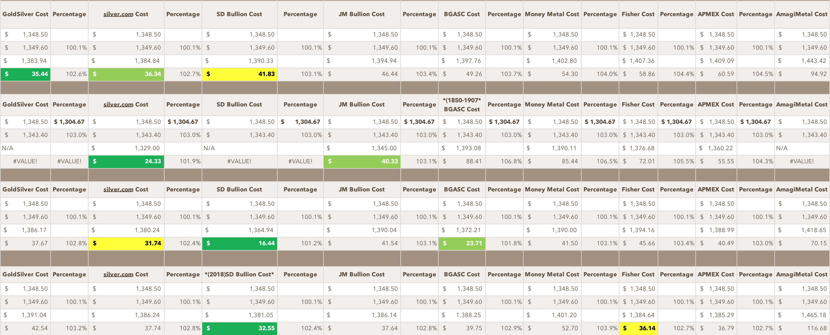
Having a little trouble with my excel at the moment but here is a screenshot of a section of the data. The array of data I need to pull from starts in C8 and goes to X41, so C8:X41. As you can see in the screen shot under each store there is a value calculation. In the above array I need to find the smallest result and return it to a summary sheet. I hope this helps and thank you for responding.
- SergeiBaklanDiamond Contributor
Benjamin,
It's hard to understand from your screenshot where which columns/rows are, but the idea is
=AGGREGATE(15,6,1/(MOD(COLUMN($C$8:$X$8)-COLUMN($C$8),2)=0)/(MOD(ROW($C$8:$C$41)-ROW($C$8),6)=0)/(C8:X41<>0)*C8:X41,1)
We check every second column and every sixth row, only to adjust from which cell to calculate.
Please see attache sample to illustrate.