Forum Discussion
luigi Pameijer
May 31, 2017Copper Contributor
Help with this "IFS" statement in office 365
I looked up how to write this statement, found a solution on the web (Example 2) see attached image
I typed the exact same information into my spreadsheet using the formula shown.
and get a different result.
I am using a iMac.
https://support.office.com/en-us/article/IFS-function-36329a26-37b2-467c-972b-4a39bd951d45
Example 2
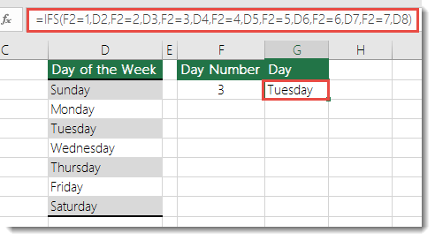
The formula in cell G7 is:
=IFS(F2=1,D2,F2=2,D3,F2=3,D4,F2=4,D5,F2=5,D6,F2=6,D7,F2=7,D8)
Why is it that the example has a result of Tuesday but I get #NAME?
Please help
Why is it that I get the result of #NAME? in the cell rateher than the correct result of Tuesday.
I was going to use this formuls to create a formula ( have spelled it out in long hand)
"ifs (the word in this cell is BUTTER) and if (the value in this cell = 2) then insert the value 55, (the word in this cell is CHEESE) and if (the value in this cell = 3) then insert the value 65, (the word in this cell is MILK) and if (the value in this cell = 1) then insert the value 35
The result I get is "#NAME?"
Whats the go?
Luigi
 Deleted
Hello Luigi,
Replying specifically to your BUTTER/CHEESE/MILK formula, the IFS formula should look like this:
=IFS(AND(A1="BUTTER",B1=2),55,AND(A1="CHEESE",B1=3),65,AND(A1="MILK",B1=1),35)
And looks like this in Excel Online:
The formula has been copied down the rows in column C as an example of the result for each combination of values.
The #N/A error occurs as there is no match for the "something is true" of MILK AND 5.
A simple way to avoid this error is to add ' TRUE,"" ' to the end of the formula, like so:
=IFS(AND(A1="BUTTER",B1=2),55,AND(A1="CHEESE",B1=3),65,AND(A1="MILK",B1=1),35,TRUE,"No match")
If each preceeding condition results in FALSE, the final 'condition' is always TRUE and you can display whatever value/text is appropriate.
Hope that helps.
 luigi PameijerCopper Contributor
Thank you Robert for your assistance.
So far none has effectivley solved the problem.
I am still resulting in the <#NAME?> as the solution to these formula.
It may be a setting in office or excel.
I find that I need to shelve this part of the project for now as I have other pressing tasks.
I will pick it up again in the weeks ahead.
Luigi
- Detlef_LewinSilver Contributor
Hello Luigi
IFS() is new in Excel 2016 (but only for Office 365 subscribers and in Excel Online).
And for your problem I would suggest a LOOKUP() formula.
- luigi PameijerCopper Contributor
Hello Detlef,
I had another go with the look up formula and still don't get it
See attachemtent
Can you give some pointers
May be I am using the wrong type of formula.
What I am trying to achieve is, from a name in a cell (8 possible options) and a number in another cell (9 options) select a value from a range of cells (in one column) to give a value.
Example if there is water in this cell and the number is 3 then select the number 25
=LOOKUP(U31=3,S31="Bones"),(U31=1,S31="Butter”),(U31=1,S31="Cheese"),(U31=1,S31="Grass"),(U31=1,S31="Meat"),(U31=1,S31="Milk"),(U31=1,S31="Water"),(U31=1,S31="Whey"),25
and then I tried this option too.
=MATCH(U31=3,S31=Bones),(U31=1,S31=Butter),(U31=1,S31=Cheese),(U31=1,S31=Grass),(U31=1,S31=Meat),(U31=1,S31=Milk),(U31=1,S31=Water),(U31=1,S31=Whey),25
- Detlef_LewinSilver Contributor
Please provide the workbook and not a photo of the workbook.
- luigi PameijerCopper ContributorHello Detlef,
I am an Office 365 subscriber.
I will try the Lookup option and let you know.
Would it go like this;
=lookup(E8=1,B3="Whey"),15,AND(E8=1,B3="Milk”),15,AND(E8=1,B3="Cheese"),15,AND(E8=1,B3="Butter"),15,AND(E8=1,B3="Meat"),20,AND(E8=1,B3="Bones"),25,AND(E8=1,B3="Grass"),15,AND(E8=1,B3="Water")- Detlef_LewinSilver Contributor
I am an Office 365 subscriber.Then IFS() should work.
For the lookup formula create a helper table in E12:F19 with the products in column E and the values in column F. Column E must be sorted in ascending order.
=LOOKUP(B3,$E$12:$F$19)
- Or CHOOSE()
- luigi PameijerCopper ContributorHello Sergei,
Detlef suggested Lookup
I will also give Choose a go
Would this formula go something like this;
=choose(E8=1,B3="Whey"),15,AND(E8=1,B3="Milk”),15,AND(E8=1,B3="Cheese"),15,AND(E8=1,B3="Butter"),15,AND(E8=1,B3="Meat"),20,AND(E8=1,B3="Bones"),25,AND(E8=1,B3="Grass"),15,AND(E8=1,B3="Water")


