Forum Discussion
Formula that can update automatically each month to show monthly KPI
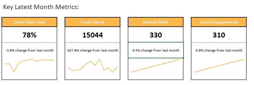
I downloaded a template with a dashboard that shows monthly metrics taken from other worksheet pages, to give an at-a-glance view of important KPI's. I don't want to use the rest of the template, so I'd like to build something similar on my own. Unfortunately, the dashboard template is locked and I can't figure out how to recreate that formula on my own. Does anyone know how to make something like this? It seems like it should be so easy, but I'm stuck on how to make the formula update with each new month of data that's added, so I don't have to reset the formula every month -- which would defeat the whole purpose.
Thanks in advance to any kind soul who might be able to save me from tearing all my hair out over this.
6 Replies
- Matt MickleBronze Contributor
This is pretty simple. This graphics are called tiles or cards and can be reproduced using a chart or sparkline and some cell formatting or the incorporation of textboxes with formulas. Do you have an example file with non-sensitive raw data that we could look at for reference? Or perhaps the original file you received? The more detail you can provide on your data structure and it's anomalies the better solution the community will be able to provide.
Before and After Examples are especially helpful.
 Caroline BartelsCopper Contributor
Hi Matt,
Thank you for your help. I'm attaching the document I'm creating based on the template. I figured out how to add text to formulas and got the %monthly change section working in the "email open rate" box on the summary tab. What I'm really stuck on is the numbers in large font in the template. Somehow the template updates those numbers whenever a new month's data is entered on the other worksheets. I can't figure out how to get Excel to find the new month's data to update automatically. If I link the summary tab cell to a single month's cell in another worksheet, I'll have to redo the formula each month, which would defeat the purpose of the quick dashboard view.- Matt MickleBronze Contributor
Please see attached for a dynamic way of calculating some of the metrics you would like. I have completed the Email Open Rate and Email Opens using Index Match Match formulas.
=INDEX(Email!$B$5:$O$29,MATCH("Open Rate",Email!$B$5:$B$29,0),MATCH(rngMonthBeg,Email!$B$5:$O$5,0))
=INDEX(Email!$B$5:$O$29,MATCH("Opens",Email!$B$5:$B$29,0),MATCH(rngMonthBeg,Email!$B$5:$O$5,0))
I also added in a few named ranges and commented your spreadsheet for better understanding.
rngToday = Today()
rngMonthBeg = EOMONTH(Z5,-2)+1
- Caroline BartelsCopper Contributor
Hi Matt,
Thank you for your help. I'm attaching the document I'm creating based on the template. I figured out how to add text to formulas and got the %monthly change section working in the "email open rate" box on the summary tab. What I'm really stuck on is the numbers in large font in the template. Somehow the template updates those numbers whenever a new month's data is entered on the other worksheets. I can't figure out how to get Excel to find the new month's data to update automatically. If I link the summary tab cell to a single month's cell in another worksheet, I'll have to redo the formula each month, which would defeat the purpose of the quick dashboard view.