Forum Discussion
Conditional formatting for an entire row based on an IF formula
Hi Edward,
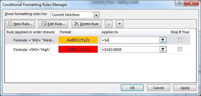
Select the whole range that you want to apply the conditional formatting on it.
For each rule, you have to put a single dollar sign $ in front of the cell address as below:
For the rule of High level, select the whole range, add a new rule, and put this formula in the formula box:
=$H1="High"
Do this for all the remaining levels!
Hope that helps
Haytham
 DeletedMar 25, 2018Not applicable
Hi Haytham,
Your solutions eradicates my entire formula. Perhaps I'm not explaining myself.
All the cells in column H are a dropdown menu. Depending on which option the user chooses from that dropdown menu, I want the individual ROW to be formatted according to that option. So if they pick "High" in H4, I want all of row 4 to be highlighted red. If they pick "Low" in H12, I want all of row 12 to be yellow. Etc.
What' I've got now isn't working.
 Haytham AmairahMar 25, 2018Silver Contributor
Hi Edward,
No matter if there is a dropdown list in column H.
You have to create a different 5 rules on the range.
Please follow the previous steps carefully!
I've created a dummy dataset to show you how it works, please find it in the attached file, and take a look at the below screenshot to figure out the technique.
Hope that helps
Haytham