spark
28 Topics
Secure Medallion Architecture Pattern on Azure Databricks (Part I)
This article presents a security-first pattern for Azure Databricks: a Medallion Architecture where Bronze, Silver and Gold each run as their Lakeflow Job and cluster, orchestrated by a parent job. Run-as identities are Microsoft Entra service principals; storage access is governed via Unity Catalog External Locations backed by the Access Connector’s managed identity. Least-privilege is enforced with cluster policies and UC grants. Prefer managed tables to unlock Predictive Optimisation, Automatic liquid clustering and Automatic statistics. Secrets live in Azure Key Vault and are read at runtime. Monitor reliability and cost with system tables and Jobs UI. Part II covers more low-level concepts and CI/CD.2.3KViews13likes0CommentsExternal Data Sharing With Microsoft Fabric
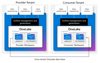
The demands and growth of data for external analytics consumption is rapidly growing. There are many options to share data externally and the field is very dynamic. One of the most frictionless and easy onboarding steps for external data sharing we will explore is with Microsoft Fabric. This external data allows users to share data from their tenant with users in another Microsoft Fabric tenant.6.8KViews3likes2CommentsHDInsight - Iceberg Open-Source Table Format
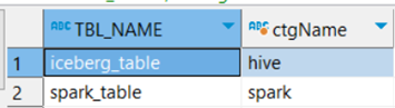
Author(s): Arun Sethia is a Program Manager in Azure HDInsight Customer Success Engineering (CSE) team. Introduction In my previous blog, we talked about leveraging Delta Lake on Azure HDInsight; this blog is dedicated to Iceberg open source table format. At this moment, HDInsight does not support Iceberg out of the box, so we will see how someone can leverage Iceberg Open Table Format in this blog. We will also see code examples to use tables from three data sources: Delta, Iceberg, and Spark native parquet files. A quick touch on Apache Iceberg - Apache Iceberg is an open-source table format that provides a transactional and versioned storage layer for big data analytics needs, originally developed to address issues in Apache Hive. It provides an alternative to Spark's default Parquet-based storage. It adds tables to compute engines, including Spark, Trino, Flink, Hive, etc., using a high-performance table format that works like a SQL table. Few silent features: Support Schema evolution without any side-effects Evolve the partition layout based on data volume and query pattern. Hidden Partition – There is no need to maintain a partition column (by transformation); it helps users not need to supply partition layout information when querying Iceberg tables. Support of time travel; useful to examine changes over time. Maintaining versions helps users to correct problems by resetting tables to a stable data version. Apache Iceberg provides an easy way to extend Spark with table specifications. In the next few sections, we will understand how to extend Spark (limited to Spark SQL) and configure the Apache Iceberg catalog with HDInsight. Spark Extension Before we jump into how to use Iceberg with HDInsight 5.0 and Spark, let us spend some time understanding a few concepts related to Spark extensions. It can help with the why and how part of the Iceberg configuration with HDInsight. Using SparkSessionExtensions provides various extension points to extend the Spark Session. The Spark SQL extension is a custom class to extend the behavior of the Spark SQL. The Spark SQL extension can be configured using the configuration property spark.sql.extensions. You can specify a comma-separated list of fully qualified class names for the extension classes you want to use in Spark SQL. With these extensions, you can extend and customize the behavior of Spark SQL. You can specify a comma-separated list of fully qualified class names for the extension classes you want to use in Spark SQL. Some common Spark SQL extensions are CSV data source, Avro data source, query optimization rules, etc. Such custom application-specific Spark configuration can be made in multiple ways; based on your deployment methods: Either by passing the configuration part of the Spark-Submit command Using the configuration magic command from Jupyter or Programmatically from the Spark job code with the SparkSession object. Spark Catalog Spark Catalog is a centralized metadata repository that provides information on data and metadata in Spark. It stores information about data stored in Spark, tables, databases, partitions, etc. It supports SQL operations on metadata, such as CREATE table, ALTER table, etc. By default, Spark comes with two catalogs, Hive and In-memory. The Hive catalog is used to store metadata in a Hive Metastore, and the in-memory catalog is used to store metadata in-memory. Spark and Hive use independent catalogs to access tables created using Spark SQL or Hive tables. A table created by Spark resides in the Spark catalog. A table created from Hive resides in the Hive catalog. We can change the Spark default catalog to the Hive catalog using the configuration property metastore.catalog.default with the value Hive. In such case, your Spark tables are managed tables in the Hive catalog and must be transaction enabled, or you can have external tables without transaction enabled. The Spark configuration property 'spark.sql.catalog' configures the list of catalogs available in Spark SQL. It allows us to configure multiple catalogs and specify the default catalog in Spark SQL, the configuration property spark.sql.defaultCatalog allows you to set the default catalog. We can create custom catalogs by implementing the Catalog interface in Spark and registering the catalog with Spark using the "spark.sql.catalog.<catalog name>" configuration parameter, where “<catalog name >” is a unique identifier for your custom catalog. In addition to managing metadata, Spark persists Spark SQL data at the warehouse directory configured using spark.sql.warehouse.dir. Iceberg Extension Iceberg core library components enable integration with compute engines like Spark, Flink, etc. These connectors are maintained in the iceberg repository and they are built for multiple versions. Iceberg provides a runtime connector for different versions of Spark. The runtime jar (iceberg-spark-runtime) is the only addition to the classpath needed to use the Iceberg open-source table format. The Iceberg Spark connector provides an extension for Spark SQL by IcebergSparkSessionExtensions class; it adds support for Iceberg tables. The extension allows users to interact with Iceberg tables in Spark SQL using DataFrame and SQL APIs for Parquet tables. The following table provides Iceberg runtime compatibility matrix w.r.t Spark version: Spark Version Latest Iceberg Support Gradle 2.4 1.1.0 org.apache.iceberg:iceberg-spark-runtime-2.4:1.1.0 3.0 1.0.0 org.apache.iceberg:iceberg-spark-runtime-3.0_2.12:1.0.0 3.1 1.1.0 org.apache.iceberg:iceberg-spark-runtime-3.1_2.12:1.1.0 3.2 1.1.0 org.apache.iceberg:iceberg-spark-runtime-3.2_2.12:1.1.0 3.3 1.1.0 org.apache.iceberg:iceberg-spark-runtime-3.3_2.12:1.1.0 Using HDInsight, you can configure the connector either part of your uber jar (as dependent jar) or part of the Spark Submit command and SQL extension part of your application code or via Spark Submit. Configure Iceberg Runtime Connector & Extension Using Spark-Submit Provide Iceberg runtime connector dependency by supplying a Maven coordinate with –packages and provide Spark SQL extension using spark configuration property. spark-submit –packages org.apache.iceberg:iceberg-spark-runtime-3.1_2.12:1.1.0 --conf spark.sql.extensions=org.apache.iceberg.spark.extensions.IcebergSparkSessionExtensions Using Application Code Provide Iceberg runtime connector as a maven dependency to your application pom.xml file. <dependency> <groupId>org.apache.iceberg</groupId> <artifactId>iceberg-spark-runtime-${spark.major.version}_${scala.major.version}</artifactId> <version>1.1.0</version> </dependency> We can use SparkConf to set up the Iceberg Spark SQL extension and Iceberg runtime connector jar. val sparkConf = new SparkConf() sparkConf.set("spark.sql.extensions", "org.apache.iceberg.spark.extensions.IcebergSparkSessionExtensions") sparkConf.set("spark.jars.packages","org.apache.iceberg:iceberg-spark-runtime-3.1_2.12:1.1.0") Use SparkConf to build the Spark Session. val spark = SparkSession .builder() .config(sparkConf) Using Jupyter Notebook %%configure { "conf": {"spark.jars.packages": "org.apache.iceberg:iceberg-spark-runtime-3.1_2.12:1.1.0", "spark.sql.extensions":"org.apache.iceberg.spark.extensions.IcebergSparkSessionExtensions" } } Iceberg Spark SQL Catalog Iceberg supplies the following Spark SQL catalog implementations: org.apache.iceberg.spark.SparkSessionCatalog – Support for Iceberg tables to Spark’s built-in catalog, and delegates to the built-in catalog for non-Iceberg tables org.apache.iceberg.spark.SparkCatalog – It supports a Hive Metastore or a Hadoop warehouse as a catalog Spark session Catalog Iceberg table supports Spark’s built-in catalog; we can configure spark_catalog to use Iceberg’s SparkSessionCatalog. The Iceberg session catalog loads non-Iceberg tables using the spark catalog (built-in catalog). The catalog type hive defines that use Hive Catalog for Iceberg tables, and non-Iceberg tables will be created in the default spark catalog. spark.sql.catalog.spark_catalog = org.apache.iceberg.spark.SparkSessionCatalog spark.sql.catalog.spark_catalog.type = hive You can provide these configurations based on your application development and deployment method set by your enterprise: If you use the Spark-Submit command from edge nodes or Livy API to submit a job, then you can use ‘conf’ parameters. From your application code, you can use the SparkConf object to set these configurations and create SparkSession using SparkConf From Jupyter notebook, you can use configure magic command as follows. %%configure { "conf": {"spark.jars.packages": "org.apache.iceberg:iceberg-spark-runtime-3.1_2.12:1.1.0", "spark.sql.extensions":"org.apache.iceberg.spark.extensions.IcebergSparkSessionExtensions", "spark.sql.catalog.spark_catalog":"org.apache.iceberg.spark.SparkSessionCatalog", "spark.sql.catalog.spark_catalog.type":"hive" } } For example, if you run this code with the above configuration, you should see `iceberg_table` created in Hive Catalog as an external table and `spark_table` in Spark Catalog as a managed table. spark.sql("""CREATE TABLE IF NOT EXISTS iceberg_table (id string, creation_date string, last_update_time string) USING iceberg""") spark.sql("""CREATE TABLE IF NOT EXISTS spark_table (id string, creation_date string, last_update_time string)""") You can use the following query on HMS to find the catalog name for `iceberg_table` and `spark_table`: SELECT t.TBL_NAME,dbc.ctgName FROM TBLS t INNER JOIN (SELECT c.Name as ctgName, d.DB_ID as dbId FROM CTLGS c , DBS d WHERE d.CTLG_NAME = c.NAME ) dbc ON dbc.dbId=t.DB_ID WHERE TBL_NAME IN ('iceberg_table','spark_table') The output will be: Custom Catalog Iceberg supports multiple data catalog types such as Hive, Hadoop, JDBC, or custom catalog implementations. These catalogs are configured using the Hadoop configuration property spark.sql.catalog.<<catalogname>> and the type of catalog using spark.sql.catalog.<<catalogname>>.type. Hive Catalog Hadoop Catalog spark.sql.catalog.<<catalogname>>=org.apache.iceberg.spark.SparkCatalogspark.sql.catalog.<<catalogname>>.type=hive spark.sql.catalog.<<catalogname>>.uri = thrift://metastore-host:port spark.sql.catalog.<<catalogname>>.warehouse=abfs://<<warehouse path>> spark.sql.catalog.iceberg_hadoop =org.apache.iceberg.spark.SparkCatalog spark.sql.catalog.iceberg_hadoop.type=hadoop spark.sql.catalog.iceberg_hadoop.warehouse=abfs://<<warehouse path>> The catalog.uri is optional; by default, it will use hive.metastore.uris from hive-site.xml (from Ambari -> Hive -> Advanced). The catalog.warehouse is optional; by default, it will use ‘Hive Metastore Warehouse directory’ from hive-site.xml (from Ambari -> Hive -> Advanced). You can provide these configurations based on your application development and deployment method set by your enterprise: If you use the Spark-Submit command from edge nodes or Livy API to submit a job, then you can use ‘conf’ parameters. From your application code, you can use the SparkConf object to set these configurations and create SparkSession using SparkConf From Jupyter notebook, you can use configure magic command as follows (in this case we are using Hadoop catalog): %%configure { "conf": {"spark.jars.packages": "org.apache.iceberg:iceberg-spark-runtime-3.1_2.12:1.1.0", "spark.sql.extensions":"org.apache.iceberg.spark.extensions.IcebergSparkSessionExtensions", "spark.sql.catalog.spark_catalog":"org.apache.iceberg.spark.SparkSessionCatalog", "spark.sql.catalog.iceberg":"org.apache.iceberg.spark.SparkCatalog", "spark.sql.catalog.iceberg.type":"hadoop", "spark.sql.catalog.iceberg.warehouse":"/iceberg/warehouse" } } Iceberg Hive Tables With Custom Catalog The current HDInsight supports Apache Hive version 3.1.1; if you want to use Iceberg tables from Hive (catalog type hive), the HiveIcebergStorageHandler and supporting classes need to be made available on Hive’s classpath. These classes are available as part of Iceberg-Hive runtime jar. You can add the Iceberg-Hive runtime jar by including the jar file to Hive’s auxiliary classpath, so it is available by default, or if you want to use Hive shell, then this can be achieved by stating so: add jar /<<path>>/iceberg-hive-runtime-1.1.0.jar; Iceberg Hive Tables using a custom catalog can be created in two ways: Using Hive DDL Command from hive-cli or beeline CREATE EXTERNAL TABLE customer ( id bigint, name string ) PARTITIONED BY ( state string ) STORED BY 'org.apache.iceberg.mr.hive.HiveIcebergStorageHandler' TBLPROPERTIES ('iceberg.catalog'='iceberg'); The Table property 'iceberg.catalog'='iceberg' set table catalog to 'iceberg'. Using Iceberg Hive Catalog Java API – Example code is available at git repository. import org.apache.iceberg.hive.HiveCatalog import org.apache.iceberg.types.Types import org.apache.iceberg.{PartitionSpec, TableProperties, Schema => IcebergSchema} import org.apache.iceberg.CatalogProperties import org.apache.spark.sql.SparkSession val catalogName = "iceberg" val nameSpace = "default" val tableName = "customer" def createTableByHiveCatalog(spark: SparkSession): Unit = { import scala.collection.JavaConverters._ // table specification starts val schema= new IcebergSchema( Types.NestedField.required(1, "id", Types.IntegerType.get()), Types.NestedField.required(2, "name", Types.StringType.get()), Types.NestedField.required(3, "state", Types.StringType.get()) ) val spec = PartitionSpec.builderFor(schema).bucket("state", 128).build() import org.apache.iceberg.catalog.TableIdentifier val tableIdentifier: TableIdentifier = TableIdentifier.of(nameSpace,tableName) val tblProperties = Map(TableProperties.ENGINE_HIVE_ENABLED->"true","iceberg.catalog"->"iceberg") // table specification ends val catalog = new HiveCatalog() catalog.setConf(spark.sparkContext.hadoopConfiguration) val properties = Map(CatalogProperties.WAREHOUSE_LOCATION->"/iceberg/warehouse/") catalog.initialize(catalogName, properties.asJava) catalog.createTable(tableIdentifier, schema, spec,s"/iceberg/warehouse/${tableName}",tblProperties.asJava) } Example - Delta, Iceberg and Spark Parquet Let us jump into the example code; in this example code, we will create sample data for Product master, Sales, and Return transactions using Mockneat. These data are stored in three file formats – Spark Parquet, Iceberg Parquet, and Delta Parquet. The scenario setup is as follows: The sample code for using Jupyter notebook is available at hdinotebookexamples. Limitation: There are limitations; at this moment, Delta Lake and Hudi currently do not support custom catalogs (out of the box). However, since Iceberg supports a custom catalog, the option is only to use spark_catalog to DeltaCatalog and create a custom catalog for Iceberg. References: https://iceberg.apache.org/ https://github.com/apache/hudi/issues/5537 HDInsight Open Table Formats: Hudi on HDInsight - https://murggu.medium.com/apache-hudi-on-hdinsight-8d981269a97a Delta Lake on HDInsight - Delta Lake on HDInsight - Microsoft Community Hub9.9KViews3likes0CommentsDelta Lake on HDInsight
Introduction Azure HDInsight is a managed, full-spectrum, open-source analytics service in the cloud for enterprises. HDInsight Apache Spark cluster is parallel processing framework that supports in-memory processing, it is based on Open-Source Apache Spark. Apache Spark is evolving; it’s efficiency and ease of use makes it a preferred big data tool among big data engineers and data scientists. There are few essential features missing from the Spark, one of them is A(Atomicity)C(Consistency)I(Isolation)D(Durability) transaction. Majority of databases supports ACID feature out of the box, when it comes to Storage layer (ADLS Gen2) it is hard to support similar level of ACID feature provided by databases. Delta Lake is a storage layer that brings ACID transactions to Apache Spark and big data workloads - for both streaming and batch operations. Delta Lake uses versioned Parquet files to store your data in your cloud storage. Apart from the versions, Delta Lake also stores a transaction log to keep track of all the commits made to the table or blob store directory to provide ACID transactions. This blog is not about Delta Lake; we will talk more about how you can leverage delta with HDInsight Spark Cluster, few code snippet and require configurations. Before we jump into code and require configurations, it is good for you check your Spark version from Ambari user interface from the HDI cluster. You need to pick the right delta lake versions based on your cluster Spark Version. The following table lists Delta Lake versions and their compatible Apache Spark versions: HDI Version Spark Version Delta Lake Version API URL 4.0 Spark 2.4.4 < 0.7.0 0.6.1 API Doc 5.0 Spark 3.1.2 1.0.x 1.0.1 API Doc HDInsight - Delta Lake Configuration Before we jump into code and configurations; we need to look into the below mentioned extendibility configurations provided by Spark: spark.sql.extensions – It is used to configure Spark Session extensions, by providing the name of the extension class. spark.sql.catalog.spark_catalog – This plugin configuration is used to configure custom catalog implementation. You can find the current catalog implementation from CatalogManager spark.sessionState.catalogManager.currentCatalog. The Spark 3.x uses SessionCatalog as default catalog. When you would like to use Delta Lake on Spark 3.x on HDI 5.0, you need to configure sql extensions and delta lake catalog with following values: Configuration Property Delta Lake Value Description spark.sql.extensions io.delta.sql.DeltaSparkSessionExtension An extension for Spark SQL to activate Delta SQL parser to support Delta SQL grammar. spark.sql.catalog.spark_catalog org.apache.spark.sql.delta.catalog.DeltaCatalog This replaces Spark’s default catalog by Delta Lake DeltaCatalog. The above configurations need to be provided as part of the Spark Configuration before any Spark session is created. Apart from the above Spark configurations, the Spark Application uber jar should provide Delta Lake dependency. Working with Spark 2.4.x with HDI 4.0 we just need to supply Delta Lake dependency, no additional spark configurations. To avoid class loading conflicts due to duplicate classes on the cluster classpath, we need to use the maven-shade-plugin to create an uber-jar with jackson dependencies. Example Code You can clone the example code from GitHub, the code is written in Scala. You can run example code using anyone of this option: Copy the application jar to the Azure Storage blob associated with the cluster. SSH to Headnode and run Spark-Submit from the headnode Or Using Livy API or Use Azure Toolkit for IntelliJ The example application will generate stdout logs and delta lake parquet files with commit logs. The output examples are listed on GitHub. Summary Delta Lake is an open-source storage framework that extends parquet data files with a file-based transaction log for ACID transactions and scalable metadata handling. Delta lake is fully compatible with Apache Spark APIs. Since the HDInsight Spark cluster is an installation of the Apache Spark library onto an HDInsight Hadoop cluster, the user can use compatible Delta Lake versions to take benefits of Delta Lake on HDInsight.5.8KViews3likes0CommentsSmart Pipelines Orchestration: Designing Predictable Data Platforms on Shared Spark
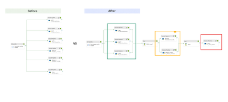
Introduction In mature data platforms, scaling compute is rarely the primary challenge. Shared, elastic Spark pools already provide sufficient processing capacity for most workloads. The harder problem is achieving predictable execution when multiple pipelines compete for the same resources. In Azure Synapse, Spark pools are commonly shared across pipelines to optimize cost and utilization. While this model is efficient, it introduces a key limitation: execution order is determined by scheduling behavior, not business priority. This post describes an orchestration pattern that makes priority explicit, allowing critical workloads to run predictably on shared Spark compute without modifying Spark code, configuration, or cluster capacity. Goal This work does not aim to optimize Spark performance. Its goal is to ensure that, when pipelines share a Spark pool: latency-sensitive workloads run first heavy backfills do not delay critical pipelines execution order is deterministic under contention All of this needed to be achieved without changes to Spark configuration, notebook logic, or cluster size. Why This Problem Occurs In a naïve orchestration model, pipelines are triggered in parallel. From Spark’s perspective: all jobs are equivalent all jobs attempt to acquire executors at the same time scheduling decisions are based on availability and timing As a result, priority is implicit and often incorrect. A heavy workload may acquire executors before a lightweight but critical one simply because it requests more resources earlier. This behavior is expected from Spark. The issue lies in orchestration, not in compute. Core Concept: Priority as Execution Ordering In shared Spark platforms, priority is enforced through execution ordering, not compute tuning. The orchestration layer controls when workloads are admitted to shared compute. Once execution begins, Spark processes each workload normally. This preserves Spark’s execution model while providing deterministic workload ordering. Step 1: Workload Classification In the demo presented in this blog, workloads are classified during configuration based on business impact: Category Description Priority example Light (critical) SLA sensitive dashboard and downstream consumers High priority , low resource weight(data volume) Medium (High) Core reporting workloads Medium priority Heavy(Best Effort) Backfills and historical computes Low priority, high resource weight(data volume) This classification is external to Spark and external to code. It represents business intent, not implementation. As a future phase, classification can be automated,for example, an agent may adjust priority based on observed failure rates or execution stability. Workload classification is expressed as orchestration metadata, for example: [ {"name":"ExecDashboard","pipeline":"PL_Light_ExecDashboard","weight":1,"tier":"Critical"}, {"name":"FinanceReporting","pipeline":"PL_Medium_FinanceReporting","weight":3,"tier":"High"}, {"name":"Backfill","pipeline":"PL_Heavy_Backfill","weight":8,"tier":"BestEffort"} ] What Runs in Each Workload Category All pipelines execute on the same shared Spark pool, but the work they perform differs in scope, data volume, and sensitivity to contention. Light workloads power SLA-sensitive dashboards and downstream consumers. Their notebooks perform targeted reads with strong filtering, limited joins, and small aggregations. Execution time is short, and overall pipeline duration is dominated by executor availability rather than computation. Medium workloads represent core reporting and analytics logic. These notebooks process larger datasets, perform joins across multiple sources, and apply aggregations that are more expensive than Light workloads but still time-bounded and business-critical. Heavy workloads are best-effort pipelines such as backfills and historical recomputation. Their notebooks scan large data volumes, apply expensive transformations, and are optimized for throughput rather than responsiveness. These workloads tolerate delay but place significant pressure on shared compute when admitted concurrently. All workloads use the same Spark pool, executor configuration, and runtime. The distinction reflects business intent and execution characteristics, not Spark tuning. Example notebooks for each category are available in the accompanying GitHub repository. Step 2: Naïve Orchestration (Baseline) The following pipeline run illustrates the baseline behavior when all workloads are triggered in parallel against a shared Spark pool. All Light, Medium, and Heavy pipelines are admitted concurrently. Executor acquisition and execution order depend on timing rather than business priority, resulting in non-deterministic behavior under contention. Although Light workloads require minimal compute, they are delayed by executor contention caused by Medium and Heavy pipelines entering the Spark pool at the same time. Step 3: Smart Orchestration (Priority-Aware) Orchestration Model The same child pipelines and notebooks are reused. The parent pipeline enforces admission order: Light (Critical) Medium (High) Heavy (Best Effort) Dependencies control admission to the Spark pool. Parallelism is preserved within a priority class. Effect on Shared Spark Light workloads enter the Spark pool without contention Medium workloads run after Light completes Heavy workloads are intentionally delayed Executor acquisition aligns with business priority Light pipelines execute first and complete before medium pipelines are admitted. Heavy workloads run last by design. No Spark configuration changes are introduced. The Spark pool, notebooks, and executor configuration are identical to the naïve run. Only the orchestration graph differs. Step 4: Impact on Light Workloads Light workloads are particularly sensitive to orchestration because their runtime is dominated by queueing time, not computation. Comparing the naïve and priority-aware runs shows that Spark execution time is unchanged, but pipeline duration improves due to earlier admission to the Spark pool and immediate executor access Naïve Execution Spark execution time: short and unchanged Pipeline duration: minutes under contention Delay caused by executor unavailability Smart Execution Spark execution time: unchanged Pipeline duration closely matches compute time Immediate access to executors The improvement comes from removing admission contention, not from increasing resources. Results and Performance Compared to naïve orchestration, priority-aware orchestration ensures that Light workloads complete in minutes rather than tens of minutes under contention, while Spark execution time itself remains unchanged. Heavy workloads no longer delay latency-sensitive pipelines, and execution order is deterministic across runs. These improvements are achieved solely by controlling admission to the shared Spark pool, without modifying Spark configuration, notebook logic, or cluster capacity. Next Steps: 1. Optimizing Heavy Workloads Once heavy workloads are isolated by priority, they can be optimized independently: retries with backoff tolerance for transient failures increased executor counts or larger pools Without admission control, these optimizations increase contention, with smart orchestration, they do not impact critical pipelines. 2. Moving Beyond Static Classification In this implementation, workload classification is static and configuration-driven, which is sufficient for stabilization. A next phase is adaptive classification: collect execution metrics and failure rates detect unstable pipelines reclassify pipelines that exceed thresholds (e.g., >20% failures in a rolling window) This prevents unstable workloads from impacting critical execution paths and makes the pipeline reliable with minimal maintenance. 3. Assisted Classification with Copilot agent At scale, priority decisions benefit from automation. A Copilot-style agent can use historical execution data to recommend classification changes, grounding decisions in observed behavior while keeping engineers in control. Example: Changing workload classification from Light to Medium Consider a pipeline initially classified as Light because it powers an SLA-sensitive dashboard and typically executes quickly with minimal resource usage. Over time, execution telemetry shows a change in behavior: The pipeline fails in 4 of the last 10 runs due to transient Spark errors Average duration has increased by 3×, even when admitted early Retry attempts amplify contention for other Light workloads Based on these signals, an automated agent flags the workload as unstable and recommends reclassifying it from Light to Medium. After reclassification: The pipeline is admitted after Light workloads but before Heavy workloads It no longer blocks latency-critical paths when retries occur Execution remains predictable, while instability is isolated from critical workloads The notebook logic and Spark configuration remain unchanged, only the workload’s admission priority is updated via orchestration metadata. This approach allows the platform to adapt to changing workload characteristics while preserving deterministic execution for critical pipelines. Conclusion Parallel execution is a default, not a strategy. In shared environments, orchestration must explicitly encode business intent rather than relying on scheduler behavior. Enforcing priority at the orchestration layer restores predictability without sacrificing efficiency and provides a foundation for adaptive, policy-driven execution as platforms evolve. Links Orchestrating data movement and transformation in Azure Data Factory - Training | Microsoft Learn How to Optimize Spark Jobs for Maximum Performance: A Complete Guide GitHub repo for notebook reference: sallydabbahmsft/Smart-pipelines-orchestration Feedback: Sally Dabbah | LinkedIn853Views2likes2CommentsOverload to Optimal: Tuning Microsoft Fabric Capacity
Co-Authored by: Daya Ram, Sr. Cloud Solutions Architect and Rafia Aqil, Could Solutions Architect Optimizing Microsoft Fabric capacity is both a performance and cost exercise. By diagnosing workloads, tuning cluster and Spark settings, and applying data best practices, teams can reduce run times, avoid throttling, and lower total cost of ownership—without compromising SLAs. Use Fabric’s built-in observability (Monitoring Hub, Capacity Metrics, Spark UI) to identify hot spots and then apply cluster- and data-level remediations. Capacity Planning For capacity planning and sizing guidance, see Plan your capacity size. Selecting the wrong SKU can lead to two major issues: Over-provisioning: Paying for resources you don’t need. Under-provisioning: Struggling with performance bottlenecks and failed jobs. To simplify this process, Microsoft provides the Fabric SKU Estimator, a powerful tool designed to help organizations accurately size their capacity based on real-world usage patterns. Run the SKU Estimator before onboarding new workloads or scaling existing ones. Combine its recommendations with monitoring tools like Fabric Capacity Metrics to validate performance and adjust as needed. Options to Diagnose Capacity Issues 1) Monitoring Hub — Start with the Story of the Run What to use it for: Browse Spark activity across applications (notebooks, Spark Job Definitions, and pipelines). Quickly surface long‑running or anomalous runs; view read/write bytes, idle time, core allocation, and utilization. How to use it From the Fabric portal, open Monitoring (Monitor Hub). Select a Notebook or Spark Job Definition to run and choose Historical Runs. Inspect the Run Duration chart; click on a run to see read/write bytes, idle time, core allocation, overall utilization, and other Spark metrics. What to look for Use the guide: application detail monitoring to review and monitor your application. 2) Capacity Metrics App — Measure the Whole Environment What to use it for: Review capacity-wide utilization and system events (overloads, queueing); compare utilization across time windows and identify sustained peaks. How to use it Open the Microsoft Fabric Capacity Metrics app for your capacity. Review the Compute page (ribbon charts, utilization trends) and the System events tab to see overload or throttling windows. Use the Timepoint page to drill into a 30‑second interval and see which operations consumed the most compute. What to look for Use the Troubleshooting guide: Monitor and identify capacity usage to pinpoint top CU‑consuming items. 3) Spark UI — Diagnose at Deeper Level Why it matters: Spark UI exposes skew, shuffle, memory pressure, and long stages. Use it after Monitoring Hub/Capacity Metrics to pinpoint the problematic job. Key tabs to inspect Stages: uneven task durations (data skew), heavy shuffle read/write, large input/output volumes. Executors: storage memory, task time (GC), shuffle metrics. High GC or frequent spills indicate memory tuning is needed. Storage: which RDDs/cached tables occupy memory; any disk spill. Jobs: long‑running jobs and gaps in the timeline (driver compilation, non‑Spark code, driver overload). What to look for Set via environment Spark properties or session config. Data skew, Memory usage, High/Low Shuffles: Adjust Apache Spark settings: i.e. spark.ms.autotune.enabled, spark.task.cpus and spark.sql.shuffle.partitions. Remediation and Optimization Suggestions A) Cluster & Workspace Settings Runtime & Native Execution Engine (NEE) Use Fabric Runtime 1.3 (Spark 3.5, Delta 3.2) and enable the Native Execution Engine to boost performance; enable at the environment level under Spark compute → Acceleration. Starter Pools vs. Custom Pools Starter Pool: prehydrated, medium‑size pools; fast session starts, good for dev/quick runs. Custom Pools: size nodes, enable autoscale, dynamic executors. Create via workspace Spark Settings (requires capacity admin to enable workspace customization). High Concurrency Session Sharing Enable High Concurrency to share Spark Sessions across notebooks (and pipelines) to reduce session startup latency and cost; use session tags in pipelines to group notebooks. Autotune for Spark Enable Autotune (spark.ms.autotune.enabled = true) to auto‑adjust per‑query: spark.sql.shuffle.partitions Spark.sql.autoBroadcastJoinThreshold spark.sql.files.maxPartitionBytes. Autotune is disabled by default and is in preview; enable per environment or session. B) Data‑level best practices Microsoft Fabric offers several approaches to maintain optimal file sizes in Delta tables, review documentation here: Table Compaction - Microsoft Fabric. Intelligent Cache Enabled by default (Runtime 1.1/1.2) for Spark pools: caches frequently read files at node level for Delta/Parquet/CSV; improves subsequent read performance and TCO. OPTIMIZE & Z‑Order Run OPTIMIZE regularly to rewrite files and improve file layout. V‑Order V‑Order (disabled by default in new workspaces) can accelerate reads for read‑heavy workloads; enable via spark.sql.parquet.vorder.default = true. Vacuum Run VACUUM to remove unreferenced files (stale data); default retention is 7 days; align retention across OneLake to control storage costs and maintain time travel. Collaboration & Next Steps Engage Data Engineering Team to Define an Optimization Playbook Start with reviewing capacity sizing guidance, cluster‑level optimizations (runtime/NEE, pools, concurrency, Autotune) and then target data improvements (Z‑order, compaction, caching, query refactors). Triage: Monitor Hub → Capacity Metrics → Spark UI to map workloads and identify high‑impact jobs, and workloads causing throttling. Schedule: Operationalize maintenance: OPTIMIZE (full or selective) during off‑peak windows; enable Auto Compaction for micro‑batch/streaming writes; add VACUUM to your cadence with agreed retention. Add regular code review sessions to ensure consistent performance patterns. Fix: Adjust pool sizing or concurrency; enable Autotune; tune shuffle partitions; refactor problematic queries; re‑run compaction. Verify: Re‑run the job and change, i.e. reduced run time, lower shuffle, improved utilization.1.2KViews2likes0CommentsEnhanced autoscale capabilities in HDInsight clusters
HDInsight now has enhanced capabilities which include improved latency, and feedback loop alongside support for recommissioning nodemanagers in case of load-aware autoscale which improves cluster utilization massively and lowers the total cost of ownership significantly.5.2KViews2likes0Comments
Efficient Log Management with Microsoft Fabric
Introduction In the era of digital transformation, managing and analyzing log files in real-time is essential for maintaining application health, security, and performance. There are many 3rd party solutions in this area allowing collecting / processing storing, analyzing and acting upon this data source. But sometimes as your systems scale, those solution can become very costly, their cost model increases based on the amount of ingested data and not according to the real resources utilization or customer value This blog post explores a robust architecture leveraging Microsoft Fabric SaaS platform focused on its Realtime Intelligence capabilities for efficient log files collection processing and analysis. The use cases can vary from simple application errors troubleshooting, to more advanced use case such as application trends detection: detecting slowly degrading performance issues: like average user session in the app for specific activities last more than expected to more proactive monitoring using log based KPIs definition and monitoring those APIS for alerts generation Regarding cost , since Fabric provides a complete separation between compute and storage you can grow your data without necessarily growing your compute costs and you still pay for the resources that re used in a pay as you go model. Architecture Overview The proposed architecture integrates Microsoft Fabric’s Real time intelligence (Realtime Hub) with your source log files to create a seamless, near real-time log collection solution It is based on Microsoft Fabric: a SAAS solution which is a unified suite integrating several best of breed Microsoft analytical experiences. Fabric is a modern data/ai platform based on unified and open data formats (parquet/delta) allowing both classical data lakes experiences using both traditional Lakehouse/warehouse SQL analytics as well as real-time intelligence on semi structured data , all in on a lake-centric SaaS platform. Fabric's open foundation with built-in governance enables you to connect to various clouds and tools while maintaining data trust. This is High level Overview of Realtime Intelligence inside Fabric Log events - Fabric based Architecture When looking in more details a solution for log collection processing storage and analysis we propose the following architecture Now let's discuss it in more details: General notes: Since Fabric is a SAAS solution, all the components can be used without deploying any infrastructure in advance, just by a click of a button and very simple configurations you can customize the relevant components for this solution The main components used in this solution are Data Pipeline Onelake and Eventhouse Our data source for this example is taken from this public git repo: https://github.com/logpai/loghub/tree/master/Spark The files were taken and stored inside an S3 bucket to simulate the easiness of the data pipeline integration to external data sources. A typical log file looks like this : 16/07/26 12:00:30 INFO util.Utils: Successfully started service 'sparkDriverActorSystem' on port 59219. 16/07/26 12:00:30 INFO spark.SparkEnv: Registering MapOutputTracker 16/07/26 12:00:30 INFO spark.SparkEnv: Registering BlockManagerMaster 16/07/26 12:00:30 INFO storage.DiskBlockManager: Created local directory at /opt/hdfs/nodemanager/usercache/curi/appcache/application_1460011102909_0176/blockmgr-5ea750cb-dd00-4593-8b55-4fec98723714 16/07/26 12:00:30 INFO storage.MemoryStore: MemoryStore started with capacity 2.4 GB Components Data Pipeline First challenge to solve is how to bring the log files from your system into Fabric this is the Log collection phase: many solutions exist for this phase each with its pros and cons In Fabric the standard approach to bring data in is by use of Copy Activity in ADF or in its Fabric SAAS version is now called Data Pipeline: Data pipeline is a low code / no code tool allowing to manage and automate the process of moving and transforming data within Microsoft Fabric, a serverless ETL tool with more than 100 connectors enabling integration with a wide variety of data sources, including databases, cloud services, file systems, and more. In addition, it supports an on prem agent called self-hosted integration runtime, this agent that you install on a VM, acts as a bridge allowing to run your pipeline on a local VM and securing your connection from on prem network to the cloud Let’s describe in more details our solution data pipeline: Bear in mind ADF is very flexible and supports reading at scale from a wide range of data sources / files integrated as well to all major cloud vendors from blob storage retrieval : like S3, GCS, Oracle Cloud, File systems, FTP/SFTP etc so that even if your files are generated externally to Azure this is not an issue at all. Visualization of Fabric Data Pipeline Log Collection ADF Copy Activity: Inside Data pipeline we will create an Activity called Copy Activity with the following basic config Source: mapped to your data sources: it can be azure blob storage with container containing the log files, other cloud object storage like S3 or GCS , log files will be retrieved in general from a specific container/folder and are fetched based on some prefix/suffix in the file name. To support incremental load process we can configure it to delete the source files that it reads so that once the files are successfully transferred to their target they will be automatically deleted from their source . On the next iteration pipeline will not have to process the same files again. Sink: Onelake/Lakehouse folder: we create ahead of time a Lakehouse which is an abstract data container allowing to hold and manage at scale your data either structured or unstructured, we will then select it from the list of connectors (look for Onelake/Lakehouse) Log Shippers: This is an optional component, sometimes it is not allowed for the ETL to access your OnPrem Vnet , in this case tools like Fluentd , Filebeat , Open Telemetry collector used to forward your application collected logs to the main entry point of the system: the Azure Blob Storage. Azcopy CLI: if you don’t wish to invest into expensive tools and all you need to copy your data in a scale/secure manner to Azure Storage, you might consider create your own log shipping solution based on the free Azcopy tool together withs some basic scripting around it for scheduling: Azcopy is a command-line utility designed for high-performance uploading, downloading, and copying data to and from Microsoft Azure Blob and File storage. Fabric first Activity : Copy from Source Bucket to Lakehouse Log Preparation Upon log files landing in the azure blob storage, EventStream can be used to trigger the Data Pipeline that will handle the data preparation and loading phase. So what is Data preparation phase’s main purpose? After the log files land in the storage and before they are loaded to the realtime logs database the KQL Database , it might be necessary to transform the data with some basic manipulations . The reasons for that might be different A Few examples Bad data formats: for example, sometimes logs files contain problematic characters like new lines inside a row (stack trace error message with new lines as part of the message field of the record) Metadata enrichment: sometimes the log file names contain in their name some meaningful data : for example file name describes the originating process name / server name , so this metadata can be lost once the file content is loaded into database Regulation restrictions: sometimes logs contain private data like names, credit card numbers, social security number etc called PII that must be removed , hashed or encrypted before the load to database In our case we will be running a pyspark notebook who reads the files from Onelake folder, fixes the new lines inside a row issue, and create new files in another Onelake folder, we call this notebook with a base parameter called log_path that defines the log files location on the Onelake to read from Fabric second Activity : Running the Notebook Log Loading Inside Data pipeline , the last step, after the transformation phase, we call again the Copy data activity but this time source and sink are differen: Source: Lakehouse folder (previous notebook output) Sink: Evenhouse specific Table (created ahead of time): it is basically an empty table (lograw) Visualization of Fabric last Activity : Loading to EventHouse In summary for this stage the log collection and preparation: we broke this into 3 data pipeline activities: Copy Activity: Read the log files from source: This is the first step of the log ingestion pipeline it is running inside our orchestrator Data pipeline. Run Notebook Activity : Transform the log files : this is the execution of a single or chain of notebooks Copy Activity : Load the log files into destination datatbase : KQL inside Evenhouse : the logs database table called lograw, it is a specific table created ahead of time inside EventHouse Database Inside The Eventhouse We needed to create a KQL database with a table to hold the raw ingested log records KQL datbase is a scalable and efficient storage solution for log files, optimized for high-volume data ingestion and retrieval. Eventhouses and KQL databases operate on a fully managed Kusto engine. With an Eventhouse or KQL database, you can expect available compute for your analytics within 5 to 10 seconds. The compute resources grow with your data analytic needs. Log Ingestion to KQL Database with Update Policy We can separate the ETL transformation logic of what happens to the data before, it reaches the Eventhouse KQL database and after that. Before it reached the database , the only transformation we did was calling during the data pipeline a notebook to handle the new lines merge logic, This cannot be easily done as part of the database ingestion logic simply because when we try to load the files with new lines as part of a field of a record , it breaks the convention and what happens is that the ingestion process creates separate table records for each new line of the exceptions stacktrace. On the other hand, we might need to define basic transformation rules: such as date formatting, type conversion (string to numbers) , parse and extract some interesting value from a String based on regular exception, create JSON (dynamic type) of a hierarchical string (XML / JSON string etc) for all these transformations we can work with what is called an update policy we can define a simple ETL logic inside KQL database as explained here During this step we create from logsraw staging table a new table called logparsed , that will be our destination final table for the log queries. Those are the KQL Tables defined to hold the log files .create table logsraw ( timestamp:string , log_level:string, module:string, message:string) .create table logsparsed ( formattedDatetime:datetime , log_level:string, log_module:string, message:string) This is the update policy that automatically converts data from, the staging table logsraw to the destination table logparsed .create-or-alter function parse_lograw() { logsraw | project formattedtime = todatetime(strcat("20", substring(timestamp, 0, 2), "-", substring(timestamp, 3, 2), "-", substring(timestamp, 6, 2), "T", substring(timestamp, 9, 8))), log_level, logmodule=module, message } .alter table logsparsed policy update @'[{ "IsEnabled": true, "Source": "logsraw", "Query": "parse_lograw()", "IsTransactional": true, "PropagateIngestionProperties": true}]' Since we don't need to retain the data in the staging table (lograw) we can define a retention policy of 0 TTL like this : .alter-merge table logsraw policy retention softdelete = 0sec recoverability = disabled Query Log files After data is ingested and transformed it lands in a basic logs table that is schematized : logparsed, in general we have some common fields that are mapped to their own columns like : log level (INFO/ ERROR/ DEBUG) , log category , log timestamp (a datetime typed column) and log message which can be in general either a simple error string or a complex JSON formatted string in which case it is usually preferred to be converted to dynamic type that will bring additional benefits like simplified query logic, and reduced data processing (to avoid expensive joins) Example for Typical Log Queries Category Purpose KQL Query Troubleshooting Looking for an error at specific datetime range logsparsed | where message contains "Exception" and formattedDatetime between ( datetime(2016-07-26T12:10:00) .. datetime(2016-07-26T12:20:00)) Statistics Basic statistics Min/Max timestamp of log events logsparsed | summarize minTimestamp=min(formattedDatetime), maxTimestamp=max(formattedDatetime) Exceptions Stats Check Exceptions Distributions logsparsed | extend exceptionType = case(message contains "java.io.IOException","IOException", message contains "java.lang.IllegalStateException","IllegalStateException", message contains "org.apache.spark.rpc.RpcTimeoutException", "RpcTimeoutException", message contains "org.apache.spark.SparkException","SparkException", message contains "Exception","Other Exceptions", "No Exception") | where exceptionType != "No Exception" | summarize count() by exceptionType Log Module Stats Check Modules Distribution logsparsed | summarize count() by log_module | order by count_ desc | take 10 Realtime Dashboards After querying the logs, it is possible to visualize the query results in Realtime dashboards, for that all what’s required Select the query Click on Pin to Dashboard After adding the queries to tiles inside the dashboard this is a typical dashboard we can easily build: Realtime dashboards can be configured to be refreshed in Realtime like illustrated here: in which case user can very easily configure how often to refresh the queries and visualization : at the extreme case it can be as low as Continuus There are many more capabilities implemented in the Real-Time Dashboard, like data exploration Alerting using Data Activator , conditional formatting (change items colors based on KPIs threshold) and this framework and capabilities are heavily invested and keep growing. What about AI Integration ? Machine Learning Models: Kusto supports out of the box time series analysis allowing for example anomaly detection: https://learn.microsoft.com/en-us/fabric/real-time-intelligence/dashboard-explore-data and clustering but if it’s not enough for you, you can always mirror the data of your KQL tables into Onelake delta parquet format by selecting OneLake availability This configuration will create another copy of your data in open format delta parquet : you have it available for any Spark/Python/SparkML/SQL analytics for whatever machine learning exploration and ML modeling you wish to explore train and serve This is illustrated here : Bear in mind , there is no additional storage cost to turn on OneLake availability Conclusion A well-designed real-time intelligence solution for log file management using Microsoft Fabric and EventHouse can significantly enhance an organization’s ability to monitor, analyze, and respond to log events. By leveraging modern technologies and best practices, organizations can gain valuable insights and maintain robust system performance and security.7.4KViews1like0Comments