query optimization
2 TopicsPostgreSQL Query Rewriting and Subqueries
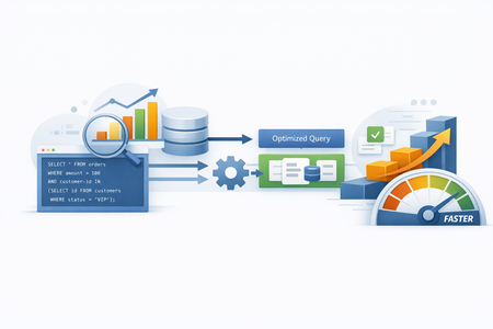
In PostgreSQL, the way a query is written has a direct impact on the execution plan the optimizer selects—and consequently on the overall performance of the system. Although the optimizer evaluates multiple plan alternatives, it can only consider strategies that the SQL structure logically allows. Suboptimal query patterns often force PostgreSQL into performing unnecessary work, such as processing more rows than needed, repeating lookups row‑by‑row or applying expensive deduplication or aggregation operations after an overly large join. By rewriting queries in more optimizer‑friendly forms, we can drastically reduce the amount of data scanned, improve join efficiency, eliminate redundant operations, and enable PostgreSQL to choose faster, more scalable execution paths. The scenarios in this document demonstrate how simple transformations—such as replacing joins with semi‑joins, pre‑aggregating large tables, or converting correlated subqueries into set‑based joins—allow PostgreSQL to leverage more efficient physical operators and achieve significant performance gains. This document explains common PostgreSQL scenarios, where rewriting a query into a subquery (or rewriting a subquery into a different form) can significantly improve performance. Each scenario includes an explanation, example rewrite, and a self-contained test script you can run. The below test was performed on a 4 vcore SKU with 128 GB storage disk. Test setup/ script: DROP TABLE IF EXISTS orders; DROP TABLE IF EXISTS customers; CREATE TABLE customers ( customer_id int PRIMARY KEY, region text NOT NULL ); CREATE TABLE orders ( order_id bigserial PRIMARY KEY, customer_id int NOT NULL REFERENCES customers(customer_id), created_at timestamptz NOT NULL ); INSERT INTO customers SELECT g, CASE WHEN g % 5 = 0 THEN 'E' ELSE 'W' END FROM generate_series(1,200000) g; INSERT INTO orders(customer_id, created_at) SELECT 1 + ((g*37) % 200000), now() - ((g % 365) || ' days')::interval FROM generate_series(1,5000000) g; CREATE INDEX orders_customer_id_idx ON orders(customer_id); ANALYZE customers; ANALYZE orders; -------------------------------------------------- Scenario 1: Semi-join filtering (JOIN → EXISTS) -------------------------------------------------- When it helps: Use this when you only need to check for the existence of related rows and do not need columns from the joined table. EXISTS allows PostgreSQL to use a semi-join strategy and avoids row multiplication. Before: SELECT DISTINCT c.customer_id FROM customers c JOIN orders o ON o.customer_id = c.customer_id WHERE c.region = 'E'; Query plan: Explanation: This query forces PostgreSQL to: • Perform a full join between customers and orders • Produce multiple rows per customer (one for each matching order) • Apply a Unique/Aggregate step to remove duplicates This results in: More rows flowing through the join Higher memory usage An expensive deduplication step Possible large hash tables or repeated nested loop iterations After: SELECT c.customer_id FROM customers c WHERE c.region = 'E' AND EXISTS ( SELECT 1 FROM orders o WHERE o.customer_id = c.customer_id ); Query plan: Explanation: The rewritten query using EXISTS, PostgreSQL can switch to a Semi Join, which has two crucial advantages: Stops scanning orders after the first match A semi‑join checks only for the existence of at least one matching row — it does not need all of them. Early termination dramatically reduces I/O. No need for DISTINCT Because no row multiplication occurs, the result is naturally unique. Why performance improves Fewer rows scanned No row explosion No sort/aggregate for DISTINCT Semi‑join is cheaper both in CPU and memory Net effect: Large reduction in join work and downstream processing. -------------------------------------------------- Scenario 2: Pre-aggregate using a subquery -------------------------------------------------- When it helps: If you only need aggregated results from a large fact table, aggregate first in a subquery and then join. This reduces join cardinality and memory usage. Before: SELECT c.region, count(*) AS order_ct FROM customers c JOIN orders o ON o.customer_id = c.customer_id GROUP BY c.region; Query plan: Explanation: The original query aggregates at the end, after joining the entire orders table with customers. The join processes millions of rows Grouping is done on the expanded join result Memory consumption grows significantly Hash join must handle a very large input After: SELECT c.region, sum(x.order_ct) AS order_ct FROM customers c JOIN ( SELECT customer_id, count(*) AS order_ct FROM orders GROUP BY customer_id ) x ON x.customer_id = c.customer_id GROUP BY c.region; Query plan: Explanation: The rewritten query aggregates orders before joining This reduces the orders table from millions of rows to just thousands (one per customer). PostgreSQL can now join a tiny, aggregated set with customers. PostgreSQL’s plan changes accordingly: • HashAggregate on orders (small output) • Join happens on significantly reduced data • Final grouping is trivial because input has already been summarized Why performance improves Drastic reduction in join input size Much smaller hash tables Fewer rows grouped at the final stage Less disk spill risk Better CPU and memory efficiency Net effect: Doing heavy work early shrinks the workload for the rest of the query. -------------------------------------------------- Scenario 3: Correlated scalar subquery → JOIN -------------------------------------------------- When it helps: Correlated scalar subqueries can behave like N+1 queries. Rewriting them as joins allows PostgreSQL to use more efficient join strategies. Before: SELECT o.order_id, (SELECT c.region FROM customers c WHERE c.customer_id = o.customer_id) AS region FROM orders o; Query plan: Explanation: Correlated Scalar Subquery A correlated subquery runs once per row of the outer table (orders). PostgreSQL has no choice but to generate a parameterized Nested Loop, which means: Scan one order Perform an index lookup into customers Repeat for every order The performance degrades linearly with table size. After: SELECT o.order_id, c.region FROM orders o JOIN customers c ON c.customer_id = o.customer_id; Query plan: Explanation: The rewritten query is a standard join removes the row‑by‑row dependency. Now PostgreSQL can: Scan both tables once Build a hash table on customers Use a Hash Join or Merge Join to match rows efficiently This transforms the execution pattern from row‑by‑row lookups to a set‑based join, which is far more efficient. Why performance improves Eliminates repeated index probes Replaces O(N) loops with a single O(N) scan + O(N) hash join Better cache utilization Fully parallelizable (semi‑correlated loops are not) Net effect: Orders and customers are processed together in a single, optimized join rather than tens or hundreds of thousands of micro‑queries. Conclusion: The rewritten queries enable PostgreSQL to choose far more efficient physical operations—such as semi‑joins, early aggregation, and set‑based hash/merge joins—dramatically reducing row processing, memory usage, and repetitive work. Overall, these improvements streamline execution paths, allowing the optimizer to operate on smaller, cleaner datasets and produce faster, more scalable query plans.551Views2likes0CommentsLessons Learned #558: What an Execution Plan XML Can Tell Us in Azure SQL Database
During a performance investigation in Azure SQL Database, we requested the execution plan to understand what the query was doing. While reviewing the evidence, the customer asked a broader question: when you open the XML of an execution plan, what do you usually look for? It was a useful question. The graphical plan helps us follow the flow of data, but the XML contains details about parameters, statistics, warnings and execution that can explain why the query behaved as it did. I do not read every attribute. I start with a few checks that help connect the customer symptom to the work performed by the query. In this article, I will walk through those checks: the type of plan, parameter values, estimated versus actual rows and statistics, missing indexes and implicit conversions, and reasons for a serial plan. The XML fragments below are simplified examples that use invented values or are adapted from examples discussed in previous articles in the Lessons Learned troubleshooting series. First check whether the plan contains execution evidence Plan What we can inspect Estimated plan Optimizer choices and estimates; the query has not executed Actual plan Plan plus available counters and warnings from that execution Cached or Query Store plan Compiled plan; normally no operator actuals for the incident For the checks involving actual rows, I request an actual execution plan. In SSMS, use Include Actual Execution Plan, or capture it using SET STATISTICS XML. Choose one method. The latter executes the query and returns its plan. The account needs the permissions to run the statement and SHOWPLAN permission. SET STATISTICS IO ON; SET STATISTICS TIME ON; SET STATISTICS XML ON; -- Execute the SELECT being investigated here. SET STATISTICS XML OFF; SET STATISTICS TIME OFF; SET STATISTICS IO OFF; Save the plan as a .sqlplan file and keep the Messages output. Record when it was captured, the parameters and the reported symptom. An execution captured later may not represent the incident. Review query literals, parameter values and object names before sharing the file. Check the right statement and its parameters A procedure or batch may contain several statements. I locate the relevant StmtSimple and its QueryPlan before interpreting a warning. StatementId and operator NodeId help keep the observations attached to the correct statement and operator; NodeId is not a stable identifier across different compilations. Next, I look at ParameterList. When available, it shows both the value used when the plan was compiled and the value used during the captured execution. <ParameterList> <ColumnReference Column="@CustomerId" ParameterDataType="int" ParameterCompiledValue="(42)" ParameterRuntimeValue="(900)" /> </ParameterList> Here, the plan was compiled with CustomerId 42 and executed with CustomerId 900. If one customer has a few orders and another has thousands, I would compare their data distribution and actual plans. Different values are a reason to investigate parameter sensitivity; they do not prove that plan reuse caused the problem. A missing runtime value means this capture did not provide it. It does not mean the runtime value was the same as the compiled value. Also, eligible queries can intentionally use different plan variants through Parameter Sensitive Plan optimization. Make the comparison match the application If the query is slow in the application but fast in SSMS, I compare the SQL text, parameter types and values, database context and session options. StatementSetOptions records options associated with compilation. <StatementSetOptions ARITHABORT="true" ANSI_WARNINGS="true" ANSI_NULLS="true" QUOTED_IDENTIFIER="true" ANSI_PADDING="true" CONCAT_NULL_YIELDS_NULL="true" NUMERIC_ROUNDABORT="false" /> A difference in context can help explain why the application and SSMS use different cached plans. I capture both rather than assuming that a fast SSMS execution represents the application. The difference itself still needs to be connected to the measured performance. Compare estimated and actual rows then inspect statistics I follow the rows through the plan and look for the first useful difference between what the optimizer expected and what the operator actually processed. <RelOp NodeId="3" PhysicalOp="Index Seek" LogicalOp="Index Seek" EstimateRows="100"> <RunTimeInformation> <RunTimeCountersPerThread Thread="0" ActualRows="20000" ActualRowsRead="80000" ActualExecutions="1" /> </RunTimeInformation> <!-- Access details omitted --> </RelOp> In this single-execution example, the operator estimated 100 rows and returned 20,000: a 200-fold underestimate. It also read 80,000 rows. I would ask why the estimate was inaccurate, and why the operator read substantially more rows than it returned. These are separate questions. For repeated or parallel operators, account for executions and threads before comparing totals. Do not add the rows from every operator to calculate the query result size. The next question is often whether the statistics were out of date. OptimizerStatsUsage identifies statistics consulted during compilation, where that information is exposed. <OptimizerStatsUsage> <StatisticsInfo Schema="[PlanXmlLab]" Table="[Orders]" Statistics="[IX_Orders_CustomerId]" LastUpdate="2026-10-10T07:00:00" SamplingPercent="20" ModificationCount="15000" /> </OptimizerStatsUsage> I check the relevant statistics object, its LastUpdate, SamplingPercent and ModificationCount together. An old timestamp or a low sampling percentage alone does not prove that it caused the estimate. Updated statistics cannot explain every discrepancy; parameter values, predicates and data distribution also matter. The XML describes the statistics consulted at compilation. To check their current state, I use sys.dm_db_stats_properties, as shown next. A subsequent update does not rewrite the evidence in an already saved plan. Check when the statistics were last updated -- Run in the affected database and set the actual table name. SELECT st.name AS statistics_name, sp.last_updated, sp.rows, sp.rows_sampled, sp.modification_counter FROM sys.stats AS st OUTER APPLY sys.dm_db_stats_properties( st.object_id, st.stats_id) AS sp WHERE st.object_id = OBJECT_ID(N'PlanXmlLab.Orders'); last_updated identifies the latest statistics update; rows and rows_sampled describe the population and sample at that update. modification_counter counts modifications to the leading statistics column since the update. Metadata visibility and permissions can affect the output. Compare this information with the same statistics object in the plan. Timestamps alone do not tell us whether the update was automatic or manual. If an update is justified, validate it in a controlled comparison using the same query and representative parameters, and capture a newly compiled plan. Read the access path alongside the row counts An Index Seek can still read many rows. I inspect SeekPredicates, any residual Predicate and ActualRowsRead where available. A broad seek range followed by filtering can explain why the rows read greatly exceed the rows returned. Likewise, a Key Lookup may be inexpensive once but expensive when repeated for thousands of rows. A scan can be the right choice when a large part of the table qualifies. The operator name is a starting point; the amount of work tells us more. For the customer, the useful explanation is concrete: this operator returned many more rows than expected, these were the statistics used, and this is the next comparison that will help establish why. That is more informative than recommending a statistics update from the timestamp alone. Read missing indexes and conversion warnings as clues Missing-index messages are easy to notice. I inspect the suggestion, but I also check whether it fits the query and the existing indexes. <MissingIndexes> <MissingIndexGroup Impact="85.0"> <MissingIndex Schema="[PlanXmlLab]" Table="[Orders]"> <ColumnGroup Usage="EQUALITY"> <Column Name="[CustomerId]" ColumnId="2" /> </ColumnGroup> <ColumnGroup Usage="INCLUDE"> <Column Name="[Amount]" ColumnId="3" /> </ColumnGroup> </MissingIndex> </MissingIndexGroup> </MissingIndexes> This example suggests a key on CustomerId with Amount included for coverage. EQUALITY and INEQUALITY describe predicate columns, while INCLUDE describes covering columns. The suggestion does not settle every detail of index design. Impact is an estimated reduction in optimizer cost. A value of 85 does not promise an 85% reduction in elapsed time. The XML may contain more suggestions than the graphical plan displays. Review existing indexes and write overhead, then measure the candidate change. Check which side of the predicate is converted <Warnings> <PlanAffectingConvert ConvertIssue="Seek Plan" Expression="CONVERT_IMPLICIT(nvarchar(50),[dbo].[Customers].[Code],0)" /> </Warnings> In this separate example, I would inspect the Code column type and the application parameter declaration. A varchar column compared with an nvarchar parameter can introduce a conversion on the column side because nvarchar has higher type precedence. The warning identifies something that may affect the plan, not a measured root cause. Whether a conversion prevents an efficient seek depends on the types, collation and expression. Test an appropriate parameter declaration while preserving required character semantics, and compare results, reads and CPU. A conversion in the projection is different from one in a search predicate. Look for an explicit reason when the plan is serial Customers sometimes ask why a query does not run in parallel when the database has multiple vCores. I look for NonParallelPlanReason in QueryPlan before assuming that more resources or a higher MAXDOP will change the result. <QueryPlan DegreeOfParallelism="0" NonParallelPlanReason="TSQLUserDefinedFunctionsNotParallelizable"> <!-- Other properties omitted --> </QueryPlan> Reason What I inspect next MaxDOPSetToOne Effective MAXDOP setting or query hint TSQLUserDefinedFunctionsNotParallelizable Scalar UDF and its inlining behavior NonParallelizableIntrinsicFunction The specific intrinsic function referenced A serial plan can be appropriate. The attribute can identify a restriction, but its absence does not fully explain the optimizer decision. Scalar UDF inlining can remove a restriction without guaranteeing parallel execution. DegreeOfParallelism="1" does not demonstrate parallel work. In Azure SQL Database, check database-scoped MAXDOP and query hints. More vCores do not override every restriction or guarantee selection of a parallel plan. Lessons learned The answer to the customer was a reading process: identify the statement and capture type, inspect parameters, compare estimated and actual work, and investigate the relevant statistics and warnings. Each observation should help us ask a better question and select a useful test. For a before-and-after comparison, preserve the query, parameters, data and relevant settings. Compare returned results, logical reads, CPU and duration. A plan describes one compilation or execution; Query Store can help establish whether the behavior changed over time. A short checklist Confirm that the plan belongs to the affected statement and execution. Check parameter values and the application context. Compare estimated and actual rows, accounting for repeated work. Inspect compilation statistics and their current update metadata. Review missing indexes, implicit conversions and serial-plan reasons. Validate the explanation with a measured comparison.