postgres
144 TopicsAzure HorizonDB: Enterprise-Ready Postgres, Engineered for the AI Era
Affan Dar, Vice President of Engineering, PostgreSQL at Microsoft Charles Feddersen, Partner Director of Program Management, PostgreSQL at Microsoft Today at Microsoft Build, we’re pleased to announce the public preview of Azure HorizonDB, a new enterprise-ready Postgres-compatible database service designed to meet the needs of modern AI applications, alongside a set of enhancements to our PostgreSQL tooling in Visual Studio Code to further streamline the developer experience. Postgres is rapidly solidifying its role as a foundational layer in modern data architectures, with accelerating adoption across industries. For developers, it has become the preferred platform for new application development, driven by its extensible architecture, mature extension ecosystem, and adherence to open standards and APIs. At the same time, enterprises are choosing Postgres to re-platform and modernize existing systems, taking advantage of its ability to support a broad range of operational workloads while enabling advanced capabilities such as vector-based data access all within a single, interoperable platform. A Postgres Platform Grounded in Security, Resilience, Scale, and Performance Azure HorizonDB is purpose-built to meet these demands, combining the flexibility developers expect from Postgres with the operational rigor enterprises require. It extends the core Postgres engine with cloud-native capabilities such as integrated identity, fine-grained network and security controls, and seamless lifecycle management, while preserving full compatibility with the open ecosystem of extensions and tools. At the same time, HorizonDB introduces advanced, natively integrated capabilities like vector data support and AI model management, enabling new classes of intelligent applications without sacrificing transactional integrity or developer productivity. These capabilities are backed by a platform designed for enterprise performance and scale. HorizonDB supports databases up to 128 TB, scales out with up to 15 read replicas for high-throughput workloads, and delivers sub-millisecond commit latency across availability zones for low-latency transactions and high availability. This combination is critical for modern applications that require consistent performance under load, including high-concurrency transactional systems, real-time AI-driven interactions, and globally distributed services. The result is a unified platform that scales from the first line of code to globally distributed, mission-critical systems. Enterprise adoption ultimately depends on trust in the platform itself. Azure HorizonDB delivers this with native integration into Microsoft Entra ID for centralized identity and access control, private endpoints for network isolation, and built-in encryption to protect data at rest and in transit. These capabilities are essential for meeting compliance requirements and enabling organizations to run mission-critical workloads with confidence, without added complexity. This foundation is critical for any application, but it becomes indispensable for AI, where secure access to data and controlled model interaction underpin every intelligent experience. Building on this, HorizonDB introduces a set of integrated AI capabilities designed to bring intelligence directly into the database. Run Fast, Memory-Efficient Vector Search with DiskANN HorizonDB brings high-performance vector search directly into Postgres through DiskANN with spherical quantization. This enables efficient, low-latency similarity search at scale while significantly reducing memory and storage overhead. Spherical quantization works by normalizing vectors and encoding them into compact representations that preserve angular distance, allowing the system to compare vectors efficiently with minimal loss in accuracy. The result is the ability to index and query large embedding datasets within the transactional engine itself, making vector search a first-class capability rather than an external dependency. "HorizonDB is compelling because it brings a PostgreSQL-compatible foundation, AI-native capabilities and enterprise-grade controls closer to the operational data layer." Jennings Balavari, Founder, Opsen AI Build Smarter Apps with Hybrid Search in Postgres HorizonDB supports hybrid search by combining vector similarity through pgvector with full-text search enabled via the pg_textsearch extension, allowing applications to match both semantic meaning and precise keyword relevance in a single query. This enables more accurate, context-aware results, such as blending intent-driven retrieval with exact term matching for search, recommendations, or RAG scenarios. By unifying these capabilities within Postgres, HorizonDB improves result quality while simplifying application design without the need for external search systems. Operationalize AI with Built-In AI Model Management Working with vectors requires models to generate, interpret, and evolve embeddings, making model lifecycle a core part of the application stack. HorizonDB introduces integrated AI model management to simplify how models are registered, versioned, and governed alongside data, including built-in support for generative GPT models and ranking models. For example, GPT models can be used to generate summaries, responses, or structured outputs directly from application data, while ranking models enable relevance scoring for search results or recommendations over vector results. By managing these models alongside the data they operate on, HorizonDB ensures consistency, traceability, and control, creating a unified environment where models and data evolve together. “As we build a multi-tenant, AI-driven commerce platform, HorizonDB has been particularly compelling in two areas: scale and how close AI capabilities are to the data itself. Running vector search, filtering, and model-driven workflows directly inside the database removes a lot of the complexity we’d normally manage across separate services." James Frawley, CIAO, ReFiBuy Bring AI into SQL with AI Functions With models managed in place, AI Functions provide a direct way to invoke them from within SQL and application logic. These functions are implemented through the azure_ai extension, which brings model invocation directly into the Postgres engine. This allows developers to embed inference into queries and transactions, eliminating the need for external orchestration. By bringing model execution closer to the data, AI Functions reduce latency, simplify application design, and make intelligent behavior a natural extension of existing Postgres workloads. "What stood out with HorizonDB is that it aligns closely with how we already think about the problem. Instead of stitching together multiple components, it brings transactional data, vector search, and AI capabilities into a single platform, which simplifies the architecture without forcing a complete rethink." Mohsin Shafqat, Director Software Engineering for Nasdaq Boardvantage®, Nasdaq Run Reliable, Event-Driven Workflows with AI Pipelines Finally, AI Pipelines operationalize these capabilities through reliable, event-driven workflows for model execution and data processing. Pipelines execute on data changes, enabling real-time asynchronous reactions without external orchestration and ensuring consistent, repeatable behavior as data evolves. Combined with model management and AI Functions, they turn embedded intelligence into something that can be run, scaled, and trusted in production, while inheriting the database’s high availability and failover characteristics for resilience. Pipelines can also be visualized and observed in real time through the Visual Studio Code extension for PostgreSQL, giving developers and operators immediate visibility into execution flow, state, and outcomes Modern Unified Experience for Data, AI, and Operations in VS Code As intelligence becomes a core part of the data platform, the developer and operator experience becomes equally critical. HorizonDB extends seamlessly into Visual Studio Code with enhanced PostgreSQL tooling that works across any Postgres deployment, not just HorizonDB. Features like AI-assisted query plans and integrated monitoring enable faster debugging and optimization, helping teams understand both database performance and AI-driven behaviors. At the same time, for Azure-based deployments, the experience is deeply integrated with platform capabilities, enabling management of networking configuration, server parameters, and server logs directly from the development environment, streamlining operations across application and infrastructure layers. Azure HorizonDB brings together enterprise-grade security, deep Postgres compatibility, and a modern AI-native data platform, all engineered for developers. It scales efficiently across workloads, from transactional systems to intelligent applications, while delivering a world-class, Azure-integrated experience in Visual Studio Code for both developers and operators. Ready to get started with Azure HorizonDB? Azure HorizonDB is now available in public preview in Australia East, Central US, Sweden Central, West US 2, and West US 3 regions. Additionally, East US, Canada Central, Indonesia Central, Italy North, Japan East, Korea Central, and Poland Central will be available in the coming weeks. You can get started today by creating a new HorizonDB instance using the Azure portal, API’s, or the Visual Studio Code extension for PostgreSQL to begin exploring these capabilities firsthand. To learn more, dive deeper into our documentation and sign-up today to try AI model management in a limited preview.Announcing new security, maintenance and analytics features for PostgreSQL at Microsoft Build 2026
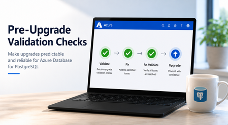
At Microsoft Build 2026, we’re announcing a major wave of PostgreSQL innovation across Azure. Alongside the public preview of Azure HorizonDB, we’re delivering a broad set of enhancements for our fully managed open-source PostgreSQL service: Azure Database for PostgreSQL flexible server. These updates span performance, analytics, security, operations, resilience and migration - helping you build faster, operate with more control, secure your workloads, and modernize with confidence. Here’s a quick tour of the top flexible server announcements at Build 2026. Feature Highlights pg_ivm Extension Defender Security assessments temporal_tables Extension Cross-tenant CMK Automatic Entra token refresh libraries New Powershell module: Az.PostgreSQLFlexibleServer More control over planned maintenance Pre-Upgrade validation checks New Built-in Grafana dashboards Chaos Studio supports Azure Database for PostgreSQL AI-assisted Oracle to PostgreSQL migration Migration Service for Azure Database for PostgreSQL improvements (EDB, AlloyDB) Performance, Scale & Analytics pg_ivm Extension Generally Available Materialized views are a useful way to optimize performance for queries that run regularly, but if underlying data becomes stale the result set needs to be recomputed. With the pg_ivm extension you can automatically maintain materialized views as the underlying data changes. This is particularly valuable for large datasets with small incremental changes that need real-time freshness, like dashboards, catalog analytics and SaaS usage reporting. We are pleased to announce the pg_ivm extension is now generally available in Azure Database for PostgreSQL. Learn more: pg_ivm. Security, Auditing & Identity Defender security assessments Preview Microsoft Defender Security Assessments for Azure Database for PostgreSQL enables continuous evaluation of your database security posture, helping identify vulnerabilities and misconfigurations across server and database configurations. Previously limited to reactive threat detection, in the latest preview release, Defender now provides proactive, risk-based insights through assessments tailored to PostgreSQL-specific best practices, delivering more relevant and actionable guidance. This helps you strengthen your security baseline, prioritize remediation, and align with best practices and compliance requirements. Learn more: https://aka.ms/Defender-Assessments-for-PG-Preview temporal_tables Extension Generally Available We’ve had many customer requests to support the temporal_tables extension, which provides built-in support for tracking and querying historical changes to data over time. Temporal tables are now generally available in Azure Database for PostgreSQL. With this extension enabled you can easily perform time-based queries, audit data changes, and maintain historical records without building custom tracking logic, simplifying application development and compliance scenarios. Learn more: temporal_tables Cross-tenant CMK Preview Azure Database for PostgreSQL now supports cross-tenant customer-managed keys (CMK) in public preview, allowing you to encrypt your data at rest using an Azure Key Vault key that resides in a separate Microsoft Entra tenant from the database service. This feature is designed for SaaS providers and enterprises that need to maintain strict separation of duties and ownership of encryption keys, enabling you to retain full control over key lifecycle management while PostgreSQL runs in a service provider’s tenant. Learn more: Data encryption at rest in Azure Database for PostgreSQL Automatic Entra token refresh libraries Preview We’re making it easier to use Entra ID authentication with Azure Database for PostgreSQL throughout the application stack by introducing new token refresh libraries for .NET, JavaScript, and Python. With Entra ID, access tokens are short-lived which can make managing their lifecycle complex in real-world applications. Developers need to be aware of token refresh and build additional handling around token expiration, connection retry, and session continuity. These new libraries remove that friction. By handling Entra token refresh seamlessly in the background, they allow applications to stay connected without interruption and with no custom logic required. The result is a simpler development experience and more resilient applications, especially for long-running or connection-heavy workloads. Across languages, the libraries provide a consistent and streamlined way to adopt secure, passwordless authentication, helping teams focus more on building their applications and less on managing authentication. Learn more: .NET, JavaScript, and Python. Operations, Maintenance & Monitoring New Powershell module: Az.PostgreSQLFlexibleServer Generally Available We’re excited to introduce the newly renamed Az.PostgreSQLFlexibleServer PowerShell module, delivering a streamlined experience for managing Azure Database for PostgreSQL with PowerShell. Building on the capabilities of the previous Az.PostgreSql module, the updated module aligns with the new features in the 2026-01-01 preview REST API. This module brings support for PostgreSQL 18, elastic clusters for scalable workloads and a range of enhancements designed to simplify management and improve performance. Whether you're provisioning new deployments or managing complex environments, this module ensures you can take full advantage of the latest platform capabilities directly from PowerShell. To learn more, visit our official documentation on PowerShell: Az.PostgreSql Module | Microsoft Learn More control over planned maintenance Generally Available We’ve seen many requests to provide more control when a maintenance update is applied to Azure Database for PostgreSQL. Sometimes when a critical workload is running you want to apply the maintenance when you’re ready. Announcing general availability this week, we’re building on the existing System and Custom maintenance window options and adding new self-service maintenance capabilities to the Azure portal. You can now reschedule upcoming maintenance updates for up to two weeks and apply maintenance on demand at a time that suits you. You can also view scheduled maintenance and review your server’s maintenance history after updates are complete. These options help you better align maintenance with your business schedules, reduce disruption during critical workload periods, and minimize the need for support-driven deferral requests. CLI and API support are coming soon. Learn more: https://aka.ms/azure-postgres-reschedule-maintenance Pre-Upgrade validation checks Preview Major version upgrades are critical for staying current with PostgreSQL features, security updates, and performance improvements, but you often discover blockers only after starting the upgrade workflow. Pre-Upgrade Validation Checks lets you validate upgrade readiness before initiating the actual upgrade by running Azure-specific upgrade checks and PostgreSQL pg_upgrade --check validations independently. The shift is simple: you can identify and fix upgrade blockers before the upgrade window begins. The feature surfaces actionable issues across configurations, extensions, dependencies, replication slots, event triggers, and other upgrade-sensitive objects. You can fix blockers, re-run validation until all checks pass, and proceed with the upgrade with greater predictability. Learn more: https://aka.ms/pg-flex-upgrade-checks New Built-in Grafana dashboards Generally Available Grafana dashboards are now built directly into the Azure portal for Azure Database for PostgreSQL - no setup, no extra cost, and no separate service to manage. You can open your PostgreSQL resource in the portal and immediately access prebuilt dashboards for key health and performance signals such as CPU, memory, storage, IOPS, connections, transactions, and availability. The key value is metrics + logs in one place. You can quickly correlate performance spikes with PostgreSQL logs, understand what changed, and troubleshoot faster using the familiar Grafana experience. Dashboards can also be customized, saved to your subscription, and shared across teams for ongoing operations. Learn more: https://aka.ms/azure-postgres-dashboards-grafana Resilience & Business Continuity Chaos Studio supports Azure Database for PostgreSQL Preview No matter how much you prepare, you only really know how good your database disaster recovery plan is when something breaks. With Chaos Studio support for Azure Database for PostgreSQL, you can simulate zone-down scenarios on PostgreSQL HA-enabled instances and validate the resilience of your mission-critical workloads. With Chaos Studio integration, you can proactively test failover behavior and gain confidence in how your applications respond to real-world zonal failures. This feature is currently available through a gated private preview. To get started, submit your subscription details using the form. Once reviewed, our team will enable the feature for your subscription, with guidance to help you begin testing. Getting started is simple: Create a Chaos Studio workspace via the Chaos Studio portal and configure your subscription, resource group, and region. Define the scope and assign the required managed identity and permissions. Review and verify your workspace setup. Browse available scenarios and select the PostgreSQL zone-down scenario. Configure the test (name, duration), then run it from My Library to begin validating failover behavior. With just a few steps, you’ll be able to simulate real-world failure conditions and gain confidence in your application’s resilience. To get started, please submit your details using this link: Private Preview Support for Chaos Studio Migration & Modernization AI-assisted Oracle to PostgreSQL migration Generally Available AI-assisted migration tooling has dramatically lowered the bar for moving between different databases and is changing the way people look at the return on investment for migration. The VS Code PostgreSQL extension comes with AI-Assisted migration tooling which converts Oracle schema and application code to Azure Database for PostgreSQL. This tooling uses GitHub Copilot, Microsoft Foundry, and custom Language Model tools to convert Oracle schema, database code and client applications into the PostgreSQL equivalents, and validates every change against a running flexible server instance. Learn more: Schema conversion, App conversion. Migration Service for Azure Database for PostgreSQL improvements (EDB, AlloyDB) Generally Available We’ve added AlloyDB and EDB Extended Server as new sources for migrating to PostgreSQL in the Azure Database for PostgreSQL Migration Service, with support for both online and offline migration support. Learn more: Migrate from AlloyDB, Migrate from EDB. Looking ahead That wraps up the Build 2026 announcements for Azure Database for PostgreSQL flexible server. There are also many great PostgreSQL technical sessions at Build this week, covering cloud-native app & AI development and migration. To find out more, here's a link to the Build session catalog for PostgreSQL sessions: https://aka.ms/Postgres-on-Azure_Build-2026. We'll continue to build out our roadmap over the coming months to deliver on your asks to improve the performance, security and stability of your PostgreSQL workloads. Check the Microsoft Blog for PostgreSQL for a regular monthly recap where we share the latest enhancements and product updates.1.6KViews2likes0CommentsLog Insights in Minutes: A Simpler pgBadger Workflow
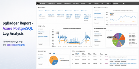
Sometimes the fastest way to understand a PostgreSQL workload is not another dashboard. It is a good log report. pgBadger is a PostgreSQL log analysis tool that turns raw PostgreSQL logs into an interactive HTML report. It helps summarize query activity, connection patterns, errors, temporary files, lock waits, autovacuum activity, and more. Earlier guidance for generating pgBadger reports from Azure Database for PostgreSQL Flexible Server focused on exporting logs through Diagnostic Settings, storing them in a storage account, and then using tools such as BlobFuse and jq to extract PostgreSQL log lines from JSON files. That workflow is still useful when customers centralize logs across multiple servers. However, if you are already using the Server logs feature in Azure Database for PostgreSQL Flexible Server, there is a much simpler path. In this post: You’ll learn how to generate a pgBadger HTML report from Azure Database for PostgreSQL Flexible Server by downloading native PostgreSQL .log files directly from the Azure portal. No storage account, BlobFuse mount, or JSON extraction required. Fast path Configure log_line_prefix . Enable Server logs for download. Download the PostgreSQL .log files. Run pgBadger with the matching prefix. Open pgbadger-report.html . Why use this workflow? With Server logs, you can download native PostgreSQL .log files directly from the Azure portal and run pgBadger locally. Older path Simpler path in this blog Diagnostic Settings → Storage account → BlobFuse → JSON extraction → pgBadger Server logs → Download .log files → pgBadger Area Older Diagnostic Settings workflow Server logs workflow Export path Diagnostic Settings to storage account Download .log files directly from the portal Format JSON payloads need extraction Native PostgreSQL .log files Extra tooling BlobFuse and jq JSON parsing None Best suited for Centralized or multi-server logging Quick per-server analysis Outcome Flexible, but more setup Faster path to pgBadger Recommended: Use the Server logs workflow when you want a fast, low-friction way to generate a pgBadger report from one Azure Database for PostgreSQL Flexible Server. When should you use this workflow? Use this workflow when... Use Diagnostic Settings when... You need a quick report for one Flexible Server. You centralize logs from many servers. You want to run pgBadger locally. You need long-term retention or workspace-level querying. You want to avoid JSON extraction. You already have automated log export pipelines. Before you start A machine where you can install or run pgBadger. A working Perl runtime. Git Bash on Windows, so the multi-line shell commands work as shown. Portal access to your Azure Database for PostgreSQL Flexible Server. Permission to update server parameters and enable Server logs. Important: pgBadger can only analyze what PostgreSQL logs capture. To populate query timing and slow-query sections in the report, enable log_min_duration_statement before collecting logs. Logs collected before that change will not include duration data. Workflow overview Task Type Rough effort Install or prepare pgBadger One-time setup per analysis machine 5–10 minutes Configure log_line_prefix One-time setup per server 2–3 minutes Enable Server logs One-time setup per server 2–3 minutes Download logs and run pgBadger Repeatable 2–5 minutes Install or prepare pgBadger on the machine where you will analyze logs. Configure log_line_prefix so pgBadger can parse each log line. Enable Server logs, so PostgreSQL logs are available for download. Download the logs and run pgBadger locally. 💡Pro tip: Start with a narrow log window first. Use one or two hourly log files, confirm the report looks right, and then expand the analysis window if needed. Step 1: Install pgBadger Before generating a report, you need pgBadger available on the machine where you plan to analyze the downloaded PostgreSQL log files. Run this on a Linux VM, WSL, or another Linux-based environment where you can install packages. Note: Azure Cloud Shell may work for quick testing, but package installation and build-tool availability can vary by session. For repeatable analysis, use a Linux VM, WSL, or another environment you control. Copy and run sudo apt-get update && sudo apt-get install -y git perl make gcc && \ git clone https://github.com/darold/pgbadger.git && \ cd pgbadger && \ perl Makefile.PL && \ make && \ sudo make install && \ pgbadger -V What good looks like: The install command completes successfully and pgbadger -V returns the installed pgBadger version. Step 2: Configure log_line_prefix This is a one-time server configuration step. The log_line_prefix parameter controls the beginning of each PostgreSQL log line. pgBadger uses this prefix to extract useful fields such as timestamp, user, database, and process ID. In the Azure portal, open your Flexible Server and go to Server parameters. Search for: Parameter log_line_prefix Set this value %m user=%u db=%d pid=%p: Then select Save. In Server parameters, confirm that the custom value is saved for log_line_prefix . Figure 1: Set log_line_prefix so pgBadger can correctly parse timestamp, user, database, and process ID from each log line. Prefix tokens Token Meaning %m Timestamp with milliseconds %u Username %d Database name %p Process ID After this change, log lines should look like this: Example log line 2026-06-22 19:00:00.070 UTC user=pgadmin db=highcpu pid=3805603: LOG: statement: SELECT 1 FROM pg_extension WHERE extname='pg_stat_statements' The matching pgBadger prefix for this log format is: Matching pgBadger prefix %m user=%u db=%d pid=%p: You will use this same value later in the pgBadger command. What good looks like: The server parameter is saved, and new PostgreSQL log lines begin with timestamp, user, database, and process ID fields that match the pgBadger prefix. Step 3: Enable Server logs for download This is also a one-time setup step. In the Azure portal, open your Flexible Server and go to Server logs. Enable: Portal setting Capture logs for download Set the retention period based on how long you want logs to remain available for download. For example, a 7-day retention period keeps logs available for download for 7 days. In Server logs, enable Capture logs for download and choose the retention window. Figure 2: Enable Capture logs for download and set a retention period long enough to cover the analysis window you want to inspect. What good looks like: After Server logs are enabled, hourly PostgreSQL log files appear in the Server logs blade and can be downloaded from the Azure portal. Once enabled, hourly log files appear in the Server logs blade. The files are named by date and hour, for example: Example log files postgresql_2026_06_22_19_00_00.log postgresql_2026_06_22_20_00_00.log Step 4: Download and organize the logs locally From the Server logs page, select the .log files for the time window you want to analyze and download them. For example, to analyze activity between 19:00 and 21:00 UTC, download: Example files to download postgresql_2026_06_22_19_00_00.log postgresql_2026_06_22_20_00_00.log On your local machine, create a folder for that analysis window. A simple convention is to use the Mon-DD format. Folder name Jun-22 Place the downloaded .log files inside that folder. Your local folder structure should look like this: Folder structure pgbadger-13.1/ pgbadger Jun-22/ postgresql_2026_06_22_19_00_00.log postgresql_2026_06_22_20_00_00.log Step 5: Generate the pgBadger report Open Git Bash from the folder where pgBadger is located. For example, if pgBadger is inside the pgbadger-13.1 folder, open Git Bash from that folder. # Action Command 1 Set the folder FOLDER=Jun-22 2 Confirm files ls -lh ./$FOLDER 3 Run pgBadger Use the full command below. Copy and run FOLDER=Jun-22 ls -lh ./$FOLDER perl -X ./pgbadger -f stderr \ --prefix '%m user=%u db=%d pid=%p:' \ ./$FOLDER/*.log \ -o ./$FOLDER/pgbadger-report.html Command breakdown Part of command Purpose perl -X ./pgbadger Runs pgBadger and suppresses non-critical Perl warnings. -f stderr Parses PostgreSQL stderr log files. --prefix '%m user=%u db=%d pid=%p:' Matches the log_line_prefix set on the server. ./$FOLDER/*.log Analyzes every .log file in the selected folder. -o ./$FOLDER/pgbadger-report.html Writes the HTML report into the same folder. When the command completes successfully, you should see output like this: Expected output Parsed 12134249 bytes of 12134249 (100.00%), queries: 26684, events: 83 LOG: Ok, generating html report... What good looks like: pgBadger finishes parsing the logs and creates pgbadger-report.html in the selected folder. Step 6: Open the report Open the generated report: Copy and run start ./$FOLDER/pgbadger-report.html The report opens in your default browser. The final report is created here: Generated report path Jun-22/pgbadger-report.html What the report can show The pgBadger report gives you a quick view into the workload shape for the selected log window. For example, in a sample run across two hourly log files, pgBadger summarized: Total number of queries. Number of unique normalized queries. Query traffic over time. Events such as errors and fatal messages. Session and connection patterns. Once the report opens, start with Global Stats to confirm the time range, total queries, normalized queries, and query peak. Figure 3: Start with Global Stats to validate the selected time range, total query count, normalized query count, and query peak. Query volume and normalized queries Many raw queries can often reduce to a smaller number of normalized query patterns. This helps identify whether the workload is spread across many different query shapes or dominated by a smaller set of repeated statements. Example: In this sample run, 26,684 queries reduced to 59 normalized query shapes. That suggests the workload is mostly a small set of repeated statements, which can help focus tuning effort. Traffic patterns The SQL Traffic section helps identify spikes, quiet periods, and workload changes over time. Figure 4: Use SQL Traffic to identify query spikes, quiet periods, and workload changes during the selected log window. Figure 5: Review the query breakdown to compare read vs. write volume and query-type distribution for the selected Server logs window. For example, if the report shows a steady baseline followed by a sharp spike, that spike can be correlated with application activity, batch jobs, synthetic tests, or operational events during the same time window. Query duration If query duration shows 0 ms or the slow query sections are empty, it usually means duration logging was not enabled when the logs were collected. In that case, pgBadger can still show query counts and events, but it cannot calculate the slowest queries, total execution time, average duration, or maximum duration. To unlock those timing sections, enable log_min_duration_statement , collect fresh logs, and rerun pgBadger. What pgBadger cannot infer from missing logs pgBadger reports are only as complete as the log data you provide. If PostgreSQL did not log duration, lock waits, temporary files, or autovacuum activity during the selected time window, pgBadger cannot reconstruct those details later. To analyze... Enable before collecting logs Slow queries log_min_duration_statement Lock waits log_lock_waits Temporary files log_temp_files Autovacuum activity log_autovacuum_min_duration Repeatable copy/paste block Reusable command block Change only FOLDER for each new analysis window. Copy and run FOLDER=Jun-22 ls -lh ./$FOLDER perl -X ./pgbadger -f stderr \ --prefix '%m user=%u db=%d pid=%p:' \ ./$FOLDER/*.log \ -o ./$FOLDER/pgbadger-report.html start ./$FOLDER/pgbadger-report.html For another date, change only this line: Update this value FOLDER=Jun-22 Examples: Example folder values FOLDER=Jun-23 FOLDER=Jul-01 FOLDER=Aug-15 Optional: Improve report quality pgBadger can only analyze the information captured in PostgreSQL logs. The default logs may be enough for query frequency, connection activity, and errors. For deeper performance troubleshooting, consider enabling additional logging parameters based on your scenario. Scenario Parameter Suggested value Notes Slow query analysis log_min_duration_statement 1000 Logs statements slower than 1 second. Short controlled test log_min_duration_statement 0 Logs every statement. Use carefully. Lock troubleshooting log_lock_waits on Helps identify lock waits. Temporary file analysis log_temp_files 0 Logs all temporary files. Autovacuum visibility log_autovacuum_min_duration 0 Useful during focused analysis. Useful parameters include: Recommended logging parameters log_lock_waits = on log_temp_files = 0 log_autovacuum_min_duration = 0 To capture query durations, configure: Duration logging log_min_duration_statement = 1000 This logs statements that run longer than 1000 milliseconds. For short test runs, you can temporarily use: Short test run only log_min_duration_statement = 0 Caution: Use log_min_duration_statement = 0 carefully on busy production servers. It logs every statement and can generate a large volume of logs. Duration matters: If duration logging is not enabled, pgBadger can still show query counts and events, but slowest-query, total duration, average duration, and maximum duration sections will be limited or empty. Common mistakes and quick fixes Symptom Likely cause Fix Report is empty Prefix mismatch Match --prefix with log_line_prefix . No duration data Duration logging was not enabled Set log_min_duration_statement before collecting logs. No files visible Server logs disabled or retention expired Enable capture and check retention. pgBadger command fails pgBadger is not in the current folder or path Run pgbadger -V to confirm installation. Common troubleshooting FAQs 1. Report is created but empty This usually means the pgBadger prefix did not match the actual log format. Check the first few lines: Copy and run head -5 ./$FOLDER/*.log Make sure the pgBadger --prefix matches the server’s log_line_prefix . 2. Report shows queries but no duration PostgreSQL logged statements but did not log durations. Enable one of the following, collect fresh logs, and rerun pgBadger: Parameter options log_min_duration_statement = 1000 # or temporarily for testing log_min_duration_statement = 0 3. No .log files are visible Confirm that Server logs are enabled: Portal setting Capture logs for download Also check the retention period. If the retention period has expired, older logs may no longer be available for download. 4. pgBadger command fails Confirm that pgBadger is available in the current folder or installed in your path. Copy and run pgbadger -V If you are running pgBadger from the local folder, use: Copy and run perl -X ./pgbadger Summary For customers already using Azure Database for PostgreSQL Flexible Server logs, the pgBadger workflow is straightforward: Install pgBadger. Configure log_line_prefix . Enable Server logs for download. Download the .log files. Place them in a local date-based folder. Run pgBadger with the matching prefix. Open pgbadger-report.html . Bottom line: Server logs give you the shortest path from Azure Database for PostgreSQL Flexible Server logs to a pgBadger report. Download the native .log files, run pgBadger with the matching prefix, and open the generated HTML report. References pgBadger - source and documentation GitHub pgBadger - project site Azure - Download server logs from the portal Flexible Server Azure - Logging concepts Flexible Server Azure - Configure server parameters via the portal PostgreSQL - log_line_prefix and logging parameters673Views2likes0CommentsLast Call: Join Live the PostgreSQL Community at POSETTE: An Event for Postgres 2026 (T‑1 week)
In just one week, the PostgreSQL community gathers again for one of the most anticipated global moments of the year: POSETTE: An Event for Postgres 2026. From June 16–18, this free and fully virtual event brings together PostgreSQL contributors, engineers, architects, and practitioners across 4 livestreams, 44 talks, and 50 speakers. But you might be wondering, why should I participate in POSETTE during the livestreams? Why join it live? Explore the schedule and choose your livestreams on the official site: Join POSETTE: An Event for Postgres 2026 Why joining live makes all the difference Yes, every talk will be available afterward. But the real value of POSETTE: An Event for Postgres 2026 happens while it is unfolding live. Be part of the virtual hallway track Participating live gives you access to the #posetteconf Discord channel, where attendees and speakers interact in real time, asking questions, sharing perspectives, and comparing approaches. This is where conversations extend beyond the talks and where ideas are challenged and refined collectively. Learn and validate your thinking in real time POSETTE is not just about listening. It is about sharpening how you think about PostgreSQL: Are you partitioning effectively? Are you approaching replication with the right mental model? Are your performance strategies aligned with how PostgreSQL actually behaves? Joining live means you can test those ideas immediately with people who build and run PostgreSQL systems at scale. Connect with practitioners solving the same problems A recurring insight from POSETTE participants is how often they discover others facing the same challenges, whether around scaling, performance, or operability. That shared experience often leads to the most valuable takeaways: not just what works, but why. What makes this year’s speakers worth your time POSETTE: An Event for Postgres 2026 brings together a diverse set of voices: PostgreSQL core contributors Engineers and architects working on production systems Specialists in performance, replication, and security Developers shaping how PostgreSQL is used in modern applications Azure Database for PostgreSQL and Azure HorizonDB engineers and experts These are practitioners who have built, debugged, and scaled real systems, and who are ready to share what they learned. Learn directly from the POSETTE speakers who are shaping PostgreSQL Bruce Momjian: understanding PostgreSQL from the inside out Read Bruce Momjian’s interview Bruce Momjian, a co-founder and core member of the PostgreSQL Global Development Group, has spent decades helping people understand how PostgreSQL really works. His session on the write-ahead log (WAL) reflects that same focus: taking something fundamental but often misunderstood and making it approachable. If you want to move beyond “using” PostgreSQL and start truly understanding its internals, how durability, recovery, and replication actually function, this is a rare opportunity to learn directly from someone who has helped build the system. Chris Ellis: making PostgreSQL practical for developers Read Chris Ellis’s interview Chris Ellis focuses on how to turn PostgreSQL’s extensive feature set into practical design choices. His session on design patterns highlights a reality many developers face: PostgreSQL offers powerful primitives, but knowing how to combine them effectively is what makes the difference. His work consistently centers on simplifying application architecture by using the database well, rather than pushing complexity into application code. Chun Lin Goh: understanding performance in real environments Read Chun Lin Goh’s interview Chun Lin Goh brings a cloud architecture and observability perspective to PostgreSQL performance. His session on performance degradation in burstable environments shows how the database behaves under real-world infrastructure constraints. This is especially relevant if you run PostgreSQL in cloud environments, where system behaviour, not just query design,can have a major impact. Derk van Veen: lessons from real-world partitioning Read Derk van Veen’s interview Derk van Veen’s work is grounded in hands-on experience operating PostgreSQL at scale. His partitioning session focuses not just on how to do things right, but also on what can go wrong,and why. Partitioning decisions often look simple early on but have long-term consequences. Learning from real mistakes and trade-offs is what makes these sessions so valuable. Hari Kiran: thinking deeply about replication Read Hari Kiran’s interview Hari Kiran’s session explores logical decoding and replication, two foundational aspects of how PostgreSQL systems scale and integrate with other systems. If your work involves distributed systems, data pipelines, or event-driven architectures, understanding these mechanics is essential. Jimmy Angelakos: uncovering subtle behavior Read Jimmy Angelakos’s interview Jimmy Angelakos focuses on practical, often overlooked aspects of PostgreSQL behavior. His session on NOTIFY highlights how features that seem simple on the surface can introduce complexity in real systems. These are exactly the kinds of nuances that can save hours or days of debugging in production. Sakshi Nasha: securing PostgreSQL for production Read Sakshi Nasha’s interview Sakshi Nasha’s work emphasizes security and production readiness. Her session on securing PostgreSQL reflects a broader shift: as PostgreSQL becomes central to more systems, security needs to be built in from the start. Her perspective is especially relevant for teams moving from development environments into production systems. Taiob Ali: connecting community and real-world usage Read Taiob Ali’s interview Taiob Ali brings a strong community-driven perspective to PostgreSQL, shaped by experience as both a practitioner and an advocate. Sessions like his often help bridge the gap between concepts and how PostgreSQL is actually used across different teams and environments. Xuneng Zhou: an independent perspective from the ecosystem Read Xuneng Zhou’s interview As an independent PostgreSQL hacker, Xuneng Zhou represents a perspective deeply rooted in the open source ecosystem itself. That viewpoint often brings a focus on fundamentals, experimentation, and how PostgreSQL evolves over time, valuable context for anyone who wants to understand not just where PostgreSQL is today, but where it is heading. This is more than a conference POSETTE: An Event for Postgres 2026 is a shared moment for the PostgreSQL community. It is an opportunity to: Learn from practitioners and contributors Challenge assumptions and refine your thinking Understand where PostgreSQL is heading next Stepping into the livestream is not just about attending talks, it is about participating in that moment. Your next step: join live If PostgreSQL is part of your work, or becoming central to it, the best way to experience POSETTE: An Event for Postgres 2026 is live. Pick the sessions that matter to you. Add the livestreams to your calendar. Join the discussion as it happens. Start here: Check out the POSETTE schedule to figure out which livestreams & which talks are for you. For any other answer you may still have, don't forget to take a look at the Ultimate Guide to POSETTE: An Event for Postgres 2026 See you live at POSETTE Whether you are exploring PostgreSQL internals, building modern applications, or scaling production systems, POSETTE: An Event for Postgres 2026 is where those conversations come together. See you at POSETTE on 16-18 June 2026.193Views1like0CommentsIntroducing Durable Functions in PostgreSQL
By Abe Omorogbe, Senior PM | Pino De Candia, Principal Software Engineer | TJ Green, Principal Software Engineer Postgres will happily store your data, run your queries, and scale with you for years. But the moment you need to do more with that data, such as running multi-step transformation, scheduling nightly rollups, generating embeddings or waiting on an approval, you hit a wall. Postgres has no built-in way to run long-lived, fault-tolerant work. That's why we built pg_durable, a new open-source PostgreSQL extension that brings durable execution directly into the database. With pg_durable, Postgres doesn’t just store your data, it runs long-lived, fault-tolerant workflows on it, with built-in retries, parallelism, scheduling, and recovery. Instead of stitching together PL/pgSQL functions or building external orchestration systems, you can now define and run resilient workflows entirely in your database, backed by Postgres' durability and high availability. And on Azure HorizonDB, pg_durable also powers AI pipelines, enabling production-ready data and AI workflows, end-to-end, right inside the database. In this post, we'll cover: The hidden trap: blocking background work What pg_durable is and the DSL that drives it How this engine powers AI pipelines on HorizonDB Sample patterns worth exploring Getting started on HorizonDB, on your laptop, and in VS Code 🚀 Want to try it out? pg_durable ships in Azure HorizonDB, Microsoft's new PostgreSQL cloud service. The HorizonDB Preview is the fastest way to try pg_durable and AI pipelines together. Get started in HorizonDB → pg_durable visualization The hidden trap: blocking background work Most Postgres teams eventually reach a point where they need to run critical tasks on their data: transformations, nightly aggregations, database maintenance workflows, embedding jobs, or multi-step business processes. So, they do the natural thing and try to keep that work inside Postgres. They end up on a journey of increasing complexity and maintenance burden. First, just run the task as a function in your database You cram the whole workflow into one PL/pgSQL function: loop, transform, call APIs, write results, return. It looks simple until you have to run it in production. One connection stays tied up the whole time. Everything runs inside one big transaction, with long locks and no visibility into partial progress. If the connection drops or the database restarts, the whole run is gone. No per-step retries. No parallelism. No scheduling. No clean way to pause for human input. When it fails, you move it outside You push the workflow into an external service: a job queue, polling workers, state tables, step coordination, retry logic, crash-recovery sweeps, and cleanup jobs. What started as a few background tasks turns into a full distributed system. Before you’ve even touched the business logic, you’re building and operating infrastructure just to coordinate work that’s still fundamentally tied to your data. Both paths are workarounds for the same missing primitive: durable, asynchronous background work that lives where your data lives. That's the gap pg_durable fills. What pg_durable actually is pg_durable is a Postgres extension that consists of a DSL (Domain specific language) and the duroxide runtime hosted in a Postgres background worker. You describe a workflow as a small SQL expression, call df.start(...), and get an instance ID back immediately. The work runs off to the side in a background worker, so it never blocks your connection or transaction, and you can check progress later with df.status() and df.result(). The execution state lives in Postgres, which means it benefits from the database’s durability, HA, backups, and recovery. Additionally, the workflow definition does not have to live in the database: your application can send it to df.start(...) over a regular Postgres connection. 2: pg_durable orchestration of worker and schema Because execution is asynchronous, pg_durable automatically breaks a workflow into discrete steps. Each step runs in its own session and transaction, commits its progress, and hands off to the next instead of keeping one giant transaction open. Steps are checkpointed in Postgres and recovered by deterministic replay, so workflows survive crashes, restarts, and failovers and resume where they left off. If a step fails, only that step retries. The whole thing is expressed through a tiny DSL of composable operators: Operator Meaning ~> Sequential. run this, then that & Parallel. fan out, wait for all | Race. fan out, take the first to finish ?> / !> Conditional. if / else @> Loop. repeat durably, survive restarts |=> Capture a step's result into a variable (reuse with $) Advanced Functions df.if() Conditional branch df.loop() Repeat statements df.join() Execute in parallel, wait for all df.http() To call an allowlisted endpoint df.wait_for_schedule() For cron-style timing df.wait_for_signal() Pause for an external event Read more about all operators and functions in pg_durable Without pg_durable vs. with pg_durable The hand-rolled version of "run three aggregations in parallel, then refresh a dashboard with retries and crash recovery" usually means 300+ lines of queue tables, polling workers, state-machine rows, per-step retry logic, crash-recovery sweeps, and cleanup jobs. Plus, the runbook to operate it. The pg_durable version: SELECT df.start( 'SELECT count(*) FROM users' & 'SELECT count(*) FROM orders' & 'SELECT sum(amount) FROM orders' ~> 'REFRESH MATERIALIZED VIEW metrics', 'refresh-dashboard' ); You write the SQL. pg_durable owns the queue, the state, the coordination, the retries, and the crash recovery. Two ways to use pg_durable 1: Use pg_durable directly (works on Azure HorizonDB or any Postgres 17) Enable it and start orchestrating: CREATE EXTENSION pg_durable; SELECT df.start($$ SELECT 'Hello, durable world!' AS message $$); -- returns an instance ID immediately; the worker runs it asynchronously From there you compose: sequential pipelines, conditional branches, races for timeout-or-result, variable passing between steps, human-in-the-loop approvals, scheduled maintenance all in SQL, close to the data, with no new infrastructure. This is the "just use Postgres" answer to a problem teams usually solve by leaving Postgres. Because it's open source under the permissive PostgreSQL License, you can clone the repo and run it on your laptop, your server, or any cloud. 2: AI pipelines (HorizonDB capability) On HorizonDB, pg_durable becomes the foundation for something even more approachable: a managed, declarative AI pipeline surface in the azure_ai extension. pg_durable gives you the durable execution engine, while the ai.* API gives you an AI-shaped model of sources, steps, sinks, and triggers that compile into a durable graph. Traditional app-tier embedding pipelines fail in predictable ways: a transient API error mid-batch with no shared checkpoint, a worker that crashes after writing chunks but before marking the parent row processed, no clean way to re-embed just the rows that changed. Move that logic into HorizonDB and the source, the steps, the sink, and the run history are all SQL, protected by the same transactions, backups, and PITR (point-in-time recovery) your data already has. A complete chunk → embed AI pipeline is one definition: SELECT ai.create_pipeline( name => 'ai_pipeline', source => ai.table_source(table_name => 'documents_ai_pipeline'), steps => ARRAY[ ai.chunk(input => 'content'), ai.embed(model => 'default-embedding', input => 'chunk_text', dimensions => 1536) ], trigger => 'on_change', sink => ai.table_sink('documents_ai_pipeline_output') ); SELECT ai.run('ai_pipeline'); Each AI step becomes a durable node, so if ai.embed() fails, ai.chunk() doesn’t run again. And with trigger => 'on_change', the pipeline runs automatically as rows change, embedding only what’s new. Add a DiskANN index on the resulting table, and you have production-ready vector search end to end, entirely inside the database. Where pg_durable fits and where it doesn't If you've used external orchestrators such as Temporal or Airflow, your first reaction is probably: why would I put control flow in my database? Fair question. pg_durable isn't trying to be a universal orchestrator. Reach for pg_durable when the workflow is tightly coupled to Postgres state. The rows it reads and writes live in the same database, it benefits from the database's own durability, backups, and PITR, and you'd rather not stand up a separate system to coordinate work that never leaves the data tier. Think: embedding pipelines, ETL jobs, scheduled maintenance, and queue-style background jobs. Reach for a dedicated orchestrator when the workflow's center of gravity is outside Postgres, fanning across heterogeneous services, or running arbitrary application logic that does not map cleanly to SQL steps, branching, loops, or HTTP calls. Get started On Azure HorizonDB CREATE EXTENSION IF NOT EXISTS pg_durable; -- Execute a simple SQL query as a durable function SELECT df.start($$ SELECT 'Hello, durable world!' AS message $$); -- Returns: a1b2c3d4 (8-character instance ID) -- Get result of a specific instance SELECT df.result(<ID>); That's it: submit, walk away, inspect. Read the documentation for more details. In VS Code, with the PostgreSQL extension A dense one-liner of ~>, &, and |=> is precise once it clicks, but the learning curve is real so flatten it with tooling. Install the PostgreSQL extension for VS Code from the Marketplace: Connect to HorizonDB or your local Postgres directly from the extension Let Copilot write the SQL. The pg-durable-sql skill turns a plain-English description ("every night, archive orders older than 90 days") into correct pg_durable syntax. Run it and watch it. The extension renders pg_durable workflows and azure_ai pipelines as live graphs, definition and each run, so you can see every step, its timing, and exactly where a failure happened. Authoring, execution, run visualization, and inspection in one window and the same tooling works against any Postgres, not just HorizonDB. On your laptop Prefer to run it yourself? Clone microsoft/pg_durable, use the Codespace prebuild or VS Code Dev Container, and add the extension on any Postgres 17. Sample patterns worth exploring The scenario guide has a full catalog of scenarios; however, these are the three I would start with. ETL Pipeline: a multi-step data transformation where each step must be completed before the next begins. Failures should stop the pipeline. SELECT df.start( 'DELETE FROM target WHERE loaded_at < now() - interval ''7 days''' -- Step 1: Cleanup old ~> 'UPDATE staging SET processed_at = now() WHERE processed_at IS NULL' -- Step 2: Mark staging ~> 'INSERT INTO target (data, source_id) SELECT data, source_id FROM staging WHERE processed_at IS NOT NULL', -- Step 3: Load 'etl-pipeline' -- Label for easy identification ); If the database restarts mid-backfill, it picks up from the last checkpointed batch, not row zero. See full example Scheduled Data Sync: poll an external API or run a job on a schedule (hourly, daily, every 30 minutes). The job should run forever and survive restarts. (See full example): -- Scheduled sync: fetch data every 30 minutes (runs forever) SELECT df.start( @> ( -- @> creates an eternal loop -- Fetch from external API (df.http( 'https://httpbingo.org/json', 'GET' ) |=> 'response') -- Store the response ~> 'INSERT INTO external_data_sync (data) VALUES ($response::jsonb)' -- Wait for next scheduled run ~> df.wait_for_schedule('*/30 * * * *') -- Cron: every 30 minutes ), 'scheduled-data-sync' ); Human-in-the-loop approval: auto-apply routine changes, pause the risky ones until a person signals approval (See full example): SELECT df.start( 'SELECT amount > 10000 AS needs_review FROM invoices WHERE id = 42' |=> 'risky' ?> ( df.wait_for_signal('invoice-42') ~> 'UPDATE invoices SET status = ''paid'' WHERE id = 42' ) !> 'UPDATE invoices SET status = ''paid'' WHERE id = 42', 'invoice-approval' ); The workflow simply waits minutes or days until a reviewer releases it with the matching signal, then resumes. The community is already running with it pg_durable launched as open source and the community is already kicking the tires. The project was a top article on Hacker News on launch day and 1.7K stars on GitHub within its first few days of initial launch. Also Franck Pachot (PostgreSQL community veteran) published an independent walkthrough, Getting Started with pg_durable: durable workflows inside PostgreSQL within days of release. The repo is actively developed, and the maintainers are reading every issue and PR. If you want improvements in our DSL ergonomics, say so. If you want an operator that doesn't exist yet, open an issue. If you've got a scenario we haven't covered, send a PR. The syntax, the docs, and the rough edges all get better when people who run Postgres in production push back. So, clone it, and build something real. If you find rough edges, open an issue or send a PR at microsoft/pg_durable. We think you'll be surprised by how much it can take. Learn more pg_durable on GitHub Durable Functions on HorizonDB AI pipelines on HorizonDB3.6KViews2likes0CommentsSELECT * FROM build2026_sessions WHERE postgres = true;
Microsoft Build 2026 is around the corner, and this year it’s shaping up to be a big one for PostgreSQL experts and enthusiasts. If you’re a developer working with Postgres, or just love exploring new database technology, there's plenty to get excited about. Microsoft’s new cloud-first evolution of PostgreSQL, Azure HorizonDB, alongside sessions featuring Azure Database for PostgreSQL, will highlight how Postgres is powering the next wave of AI-driven applications. A new horizon in Postgres Build 2026 arrives at a time when the role of databases in modern apps is evolving rapidly. From enabling AI model integration to scaling seamlessly across the cloud, PostgreSQL developers today are dealing with more complex demands than ever. That’s why Azure HorizonDB – Microsoft’s new cloud-native PostgreSQL service – is generating so much buzz ahead of Build. What is Azure HorizonDB? In short, it’s a reimagined version of PostgreSQL designed for cloud-scale performance and AI-era workloads. Azure HorizonDB, introduces a distributed architecture that decouples compute and storage, delivering sub-millisecond latencies and three times the throughput of self-managed Postgres at massive scale. It aims to preserve Postgres’s beloved features and SQL ecosystem while adding next-generation capabilities: built-in vector indexing for high-speed AI/ML retrieval, the ability to run AI models and vector operations directly in the database, and multi-zone replication for resilience. For Postgres developers, this means less time stitching together external data stores or machine learning services – and more time building powerful apps on a unified platform that’s both familiar and built for the future. The bottom line: Microsoft Build 2026 is an ideal opportunity for developers to see Azure HorizonDB in action, learn best practices for modern PostgreSQL architectures, and understand how to leverage Postgres in new scenarios like generative AI and multi-agent applications. Read on for a rundown of sessions covering these topics, complete with what you’ll learn from each one. Top sessions for PostgreSQL databases on Azure Below are key sessions tailored for PostgreSQL users and those interested in Azure HorizonDB, with session types and highlights of what you’ll gain by attending. 🎤 Breakout: From Rows to Reasoning: Designing Databases for AI Apps and Agents (BRK223, 45 min, in-person and digital options) Discover how to architect databases that can power tomorrow’s intelligent applications. This technical breakout will show how AI-ready databases can move beyond plain transactions. You’ll see live demos of integrating transactional, analytical, and vector data in one unified platform, with Azure’s new database capabilities, including Azure HorizonDB. Learn how to simplify your stack by eliminating separate analytics engines or vector stores. The session will highlight patterns that reduce data movement and latency so your apps can efficiently reason over live data with minimal complexity. 🧪 Hands-on lab: Create Advanced Postgres-Powered Agentic Apps with Azure HorizonDB (LAB511, 75 min, in person and digital options) Roll up your sleeves and get hands-on building a real multi-agent AI application with Postgres. In this advanced lab, you’ll create a production-ready AI agent powered by Azure HorizonDB as an all-in-one data, search, and intelligence layer. Experiment with retrieval-augmented generation (RAG) by combining semantic vector search (DiskANN) with traditional SQL queries right inside the database. Implement hybrid search and agent workflows without resorting to external vector databases or glue code – thanks to HorizonDB’s built-in vector indexing and in-database AI model capabilities. This lab is perfect for developers who want to experience how HorizonDB can simplify your stack and boost performance for AI-driven apps. Multiple hands-on labs are offered to suite your schedule. 💻 Demo: Simplify App Dev with Cloud-Native PostgreSQL in Azure HorizonDB (DEM364, 25 min, in-person and digital options) See how to cut your development time and complexity with built-in AI and search features in Postgres. This fast-paced demo shows how Azure HorizonDB helps eliminate the need for separate search engines and AI services by pulling those capabilities straight into PostgreSQL. Expect to learn how you can run hybrid vector + keyword queries using SQL, integrate AI models directly from within the database, and apply full-text search (BM25) and semantic ranking to get smarter results. If you’re eager to deliver intelligent apps faster, with fewer moving parts, this session will show how HorizonDB simplifies your architecture without sacrificing performance. ⚡Lightning Talk: Cloud-Native PostgreSQL, Rebuilt for Scale: Azure HorizonDB (LTG413, 15 min, in-person only) Get a rapid-fire introduction to the architecture behind HorizonDB’s eye-popping performance. This short talk dives into how HorizonDB re-architects core PostgreSQL to deliver effortless scale out and blazing speed. Learn how decoupled compute and storage, predictive caching, and multi-region replication combine to achieve sub-millisecond query latencies and 3× higher throughput than standard Postgres. If you care about performance tuning and high-scale database design, don’t miss this quick primer on the tech under HorizonDB’s hood. 👥 Interactive Table Talk: Scaling PostgreSQL for AI Apps: Patterns and Tradeoffs (TT622, 45 min, in-person only) Bring your questions and ideas to this collaborative discussion. In this open round-table session with community and Microsoft experts, you’ll explore architecture patterns for scaling PostgreSQL to meet the demands of agent-based and AI-driven applications. Discuss real-world strategies for handling vector embeddings in Postgres, unifying relational and document data, integrating with AI models, and more. Compare the trade-offs between different scaling approaches – from monolithic to microservices, sharding strategies, and new technologies like HorizonDB – and learn where each design shines or struggles in production. Come ready to share your experiences and learn from others in the room. ▶️ On-Demand: Smarter PostgreSQL Migrations to Power Modern, Intelligent Apps (OD822, 30 min, digital only) Planning to migrate to Postgres or move your databases to Azure? Start here. This on-demand session focuses on new tools and proven strategies to migrate large-scale databases to Azure Database for PostgreSQL quickly and safely. You’ll see AI-assisted migration tools in action that minimize downtime and risk when moving terabytes of data. Just as importantly, you’ll learn how migrating to Azure unlocks advanced capabilities – from boosted performance and enhanced security to AI-ready features – helping you turn your newly migrated data into intelligent apps and services. On-demand session will be available to stream on the first day of Build. Meet the team: PostgreSQL expert meetups If you’re attending Build in person, stop by the Expert Meetup (EMU) area and head to the relational cloud databases booth. This is your chance to talk directly with the engineers and product teams behind PostgreSQL on Azure. Bring your questions about architecture decisions, scaling patterns, migrations, AI workloads, or anything else on your mind. Whether you want to sanity-check a design, dig deeper into something you saw in a session, or give direct feedback, the EMU space is designed for exactly that convo. How to get the most out of Build (and what to do next) With so much great content lined up, how do you decide where to start? It really depends on what you’re most excited about: Curious about AI and agentic apps: Start with From Rows to Reasoning, then go deeper with the Simplify App Dev with HorizonDB demo or get hands-on at the Azure HorizonDB labs to see how these ideas work in practice. Performance and scale are your focus: The short Lightning Talk on HorizonDB’s cloud-native architecture and the Table Talk on scaling Postgres will both provide unique insights and pro tips for running Postgres at massive scale. Planning a migration to PostgreSQL on Azure: Watch the Smarter PostgreSQL Migrations on-demand session to learn how to migrate large workloads with minimal downtime, and the benefits you can unlock after moving to Azure. Looking for real answers to your specific questions: Make time for the PostgreSQL Expert Meetup area to connect directly with the team. No matter which sessions you choose, Build 2026 promises to be an exciting event for the PostgreSQL developer community. Browse the session catalog, save the sessions that match your interests, and we’ll see you at Build.908Views2likes0CommentsDemystifying LWLock: MultiXact SLRU Wait Events in Azure Database for PostgreSQL
What Is the MultiXact Subsystem? Before diving into the wait events, it helps to understand what PostgreSQL is protecting. When a single transaction modifies a row, PostgreSQL stores that transaction's ID (XID) directly in the row header's xmax field. Simple and fast. But what happens when two or more transactions need to hold locks on the same row simultaneously? For example: Two sessions run SELECT ... FOR KEY SHARE on the same row, OR A SELECT ... FOR UPDATE session encounters a row already locked by a foreign key check (FOR KEY SHARE), OR Multiple sub-transactions created by SAVEPOINT all reference the same row In these cases, PostgreSQL cannot store two XIDs in a single xmax field. Instead, it creates a MultiXact ID (MXID) — a composite identifier that points to a list of all involved transaction IDs. These mappings are stored in two on-disk structures: pg_multixact/offsets/ — maps each MXID to its position in the member's file pg_multixact/members/ — stores the actual list of member XIDs To avoid reading these files from disk on every row visibility check, PostgreSQL caches them in memory using a SLRU (Simple Least Recently Used) cache — a small, fixed-size ring buffer with just 8 buffer slots by default (64 KB) for offsets and 16 slots (128 KB) for members. Each of those buffer slots is protected by an LWLock (Lightweight Lock). And that LWLock is exactly where the bottleneck hides. The Core Insight: Cache Hits and Lock Contention are not mutually exclusive This is the most important concept in this entire post: pg_stat_slru measures I/O misses. pg_stat_activity wait events measure lock contention. Here is what actually happens at the microsecond level: Session A: Needs MXID 5,000,023 → Page is in SLRU cache (blks_hit++) → LWLock is needed on buffer slot 3 → Session B already holds that LWLock → Session A WAITS → wait_event = 'MultiXactOffsetSLRU' recorded The cache is warm, the page is in memory, but what happens when 50 concurrent sessions suddenly all need that same buffer slot's LWLock? Only one request can hold the LWLock at a time. Every session that queues behind the lock holder generates a wait event record, all while no disk I/O is occurring. What Triggers MultiXact SLRU Wait Events? Below are the scenario's which could trigger MultiXact SLRU Wait Events. Thundering Herd — Mass Concurrent Row Locking When dozens or hundreds of sessions simultaneously attempt to lock the same small set of rows, PostgreSQL must create and resolve MXIDs at high frequency. Each resolution requires an SLRU lookup. When all lookups target the same few SLRU pages, the buffer lock becomes a serialization point. A classic reconnect avalanche triggered when the connection pool detected server slowness and all clients retried simultaneously. Foreign Key FOR KEY SHARE vs. FOR UPDATE Conflicts This is one of the most common hidden triggers. Every time a child row is inserted or updated, PostgreSQL implicitly acquires FOR KEY SHARE on the referenced parent row to prevent the parent from being deleted. If another session simultaneously holds FOR UPDATE on that same parent row, PostgreSQL must combine both lock modes into a new MXID: -- Session A (updater): SELECT * FROM orders WHERE id = 1 FOR UPDATE; -- Session B (child inserter — FK check): INSERT INTO order_items (order_id, amount) VALUES (1, 99.00); -- Implicitly: SELECT * FROM orders WHERE id = 1 FOR KEY SHARE; -- PostgreSQL creates MXID combining both transactions → SLRU write SAVEPOINT and Sub-transaction Churn Every SAVEPOINT creates a sub-transaction XID. ORM frameworks and JDBC drivers with autosave=always silently wrap every statement in a SAVEPOINT, generating sub-XIDs that accumulate rapidly. When these sub-XIDs reference the same rows across concurrent sessions, MXID creation accelerates. Each exception handler internally creates a SAVEPOINT, even when no explicit savepoint is declared. Idle Sessions Holding MXID References Open Long-running idle-in-transaction sessions hold their MXID references open, preventing PostgreSQL's autovacuum from cleaning up old multixact entries. As the MXID space grows without cleanup, the SLRU cache (fixed at 8 pages) cannot hold all active pages simultaneously. New MXID lookups begin evicting cached pages, and under concurrency the eviction/reload cycle itself creates LWLock contention. VACUUM FREEZE During High Concurrency When autovacuum runs VACUUM FREEZE to prevent MXID wraparound, it reads and resolves every MXID on every row in the table. During this process it holds SLRU buffer locks for each lookup. Concurrent application sessions needing the same SLRU pages must wait; generating MultiXactOffsetSLRU wait events even when the underlying cause is a routine maintenance operation. How to Diagnose This in Real Time Step 1: Confirm Active Wait Events Start by querying pg_stat_activity to confirm which sessions are actively waiting on MultiXact SLRU events. Use \watch 1 to refresh every second since SLRU LWLocks are held for microseconds and brief spikes can be missed. Pay close attention to the wait_event column, MultiXactOffsetSLRU and MultiXactMemberSLRU indicate pure lock contention on cached pages, while MultiXactOffsetBuffer indicates the page was evicted from cache and is being reloaded from disk. SELECT pid, wait_event_type, wait_event, state , now() - query_start AS duration, left(query, 100) AS query FROM pg_stat_activity WHERE wait_event IN ( 'MultiXactOffsetSLRU', 'MultiXactMemberSLRU', 'MultiXactOffsetBuffer' ) ORDER BY duration DESC; Step 2: Distinguish Lock Contention From Disk I/O Once wait events are confirmed, determine whether the root cause is cache under sizing (disk I/O problem) or LWLock queue depth (lock contention problem). These look identical in pg_stat_activity but require completely different fixes. Query pg_stat_slru and focus on the blks_read and blks_zeroed columns. A blks_read = 0 alongside active wait events is the definitive signature of pure lock contention: the cache is warm but the LWLock protecting each buffer slot is the bottleneck. SELECT name, blks_hit, blks_read, blks_zeroed, flushes , ROUND(100.0 * blks_hit / NULLIF(blks_hit + blks_read, 0), 2) AS hit_pct FROM pg_stat_slru WHERE name LIKE 'MultiXact%'; Interpretation Meaning blks_read = 0 AND wait events are present Pure lock contention — the cache is warm, the lock is the bottleneck blks_read > 0 AND wait events are present Cache miss + lock contention — the SLRU cache is undersized blks_zeroed are increasing rapidly High MXID creation rate — inspect application pattern issues flushes are high (2,000+) Frequent checkpoint SLRU flushes holding an exclusive lock Step 3: Check MXID Age and Identify Hot Tables A high MXID age means autovacuum is not keeping pace with MXID creation. This causes the MXID space to span far more SLRU pages than the 8-slot cache can hold, directly worsening lock contention. Check MXID age at both the database and table level. Any database approaching 1.5 billion should be treated as a critical incident. At the table level, focus on tables with the highest mxid_age combined with high row counts and stale last_autovacuum timestamps — these are your primary VACUUM FREEZE targets. -- Database-level MXID age (watch for values > 1 billion) SELECT datname, mxid_age(datminmxid) AS mxid_age FROM pg_database ORDER BY mxid_age DESC; -- Table-level — find the worst offenders SELECT relname, mxid_age(relminmxid) AS mxid_age , pg_size_pretty(pg_total_relation_size(oid)) AS table_size, n_live_tup FROM pg_stat_user_tables t JOIN pg_class c USING (relname) WHERE c.relkind = 'r' ORDER BY mxid_age DESC LIMIT 10; Step 4: Find Queries Driving MXID Creation Once the hot tables are identified, use pg_stat_statements to pinpoint the specific queries generating MXIDs at a high rate. Focus on queries using FOR UPDATE, FOR KEY SHARE, or FOR SHARE, as these are the direct triggers for concurrent row locking. Also watch for INSERT-heavy workloads on child tables with FK references, as these implicitly acquire FOR KEY SHARE on parent rows and are a common hidden driver of MXID creation. SELECT left(query, 200) AS query, calls, mean_exec_time::numeric(10,2) AS avg_ms FROM pg_stat_statements WHERE query ILIKE '%for update%' OR query ILIKE '%for key share%' OR query ILIKE '%for share%' ORDER BY calls DESC LIMIT 10; Step 5: Catch Long-Running Idle Transactions Idle-in-transaction sessions are one of the most damaging contributors to SLRU contention. They hold row-level locks while doing nothing, preventing autovacuum from cleaning up MXIDs and forcing other sessions to queue on the same SLRU pages indefinitely. Query pg_stat_activity filtered to idle-in-transaction states and focus on sessions idle for more than 2 minutes; these are almost always stuck client tool connections (DBeaver, pgAdmin) or misbehaving application threads that opened a transaction and never committed. SELECT pid, usename, application_name, state, now() - xact_start AS txn_age , now() - state_change AS idle_duration, left(query, 100) AS last_query FROM pg_stat_activity WHERE state IN ('idle in transaction', 'idle in transaction (aborted)') AND now() - state_change > interval '2 minutes' ORDER BY idle_duration DESC; Fixes and Mitigation Strategies Terminate long-running idle-in-transaction sessions The fastest way to break the contention cycle during an active incident is to terminate sessions holding locks while idle. This immediately releases row-level locks, unblocks autovacuum, and allows MXID cleanup to resume. Always preview before terminating to avoid disrupting legitimate long-running batch jobs. -- Preview candidates first SELECT pid, usename, application_name, now() - state_change AS idle_duration FROM pg_stat_activity WHERE state = 'idle in transaction' AND now() - state_change > interval '5 minutes' ORDER BY idle_duration DESC; --then run the terminate SELECT pg_terminate_backend(pid) FROM pg_stat_activity WHERE state = 'idle in transaction' AND now() - state_change > interval '5 minutes'; Set timeouts to prevent recurrence After immediate relief, set timeouts to automatically kill idle-in-transaction sessions before they accumulate again. Both parameters take effect immediately via pg_reload_conf() with no server restart required. Choose values appropriate to your workload, use more aggressive for high-concurrency OLTP, more lenient for batch or reporting workloads. ALTER SYSTEM SET idle_in_transaction_session_timeout = 'XXmin'; ALTER SYSTEM SET statement_timeout = 'XXmin'; SELECT pg_reload_conf(); VACUUM FREEZE the most affected table Running VACUUM FREEZE on the tables identified in Step 3 immediately clears old MXIDs from row headers, replacing them with frozen values that never require SLRU lookups. This directly reduces SLRU page access and LWLock contention. For very large tables, use INDEX_CLEANUP FALSE on the first pass for speed, then run a full vacuum during off-peak hours. VACUUM FREEZE VERBOSE your_hot_table; Connection pooling Connection pooling is the most impactful long-term fix for preventing thundering herd connection storms. PgBouncer in transaction mode absorbs connection spikes at the pooler layer, ensuring PostgreSQL never sees more simultaneous sessions than the pool size, and directly reducing the number of concurrent MXID lookups and SLRU LWLock contention. On Azure PostgreSQL Flexible Server, PgBouncer is available as a built-in feature. Simply enable it via Server Parameters (pgbouncer.enabled = ON) and connect on port 6432. No separate installation is required. # Key PgBouncer settings for OLTP workloads pool_mode = transaction # Release connection after each transaction default_pool_size = 100 # Real PG connections per database/user pair max_client_conn = 5000 # Total clients PgBouncer will accept Conclusion MultiXact SLRU wait events are deceptive. A server can show 100% cache hit ratio, nominal disk I/O, and moderate CPU, all while simultaneously stalling hundreds of sessions on a lock held for microseconds. The cache appears healthy, and the problem is invisible... until sessions start piling up. The single most important diagnostic insight is this: pg_stat_slru measures I/O efficiency. pg_stat_activity measures lock contention. A 100% hit ratio does not mean there are no problems, it means the bottleneck is the lock protecting the cached page, not the cache itself. Once you know this, the path forward is clear. Use pg_stat_slru and pg_stat_activity together, never in isolation. Track mxid_age proactively, and do not wait for autovacuum to raise the alarm. Eliminate idle-in-transaction sessions before they become lock holders. Use the weakest lock mode that satisfies your application's consistency requirements. Use FOR NO KEY UPDATE instead of FOR UPDATE wherever possible. And deploy PgBouncer (available as a built-in feature on Azure Database for PostgreSQL Flexible Server) to absorb connection storms before they reach the SLRU layer. MultiXact contention is not inevitable. It is the compounded result of concurrent locking patterns, under-tuned autovacuum, and unbounded connection growth, all of which are fully controllable. The earlier you instrument for it, the less likely it becomes an incident.Real-World Success Stories with PostgreSQL on Azure
Organizations rarely leap into cloud migrations or AI-powered systems overnight. They progress in deliberate stages, establishing a reliable data foundation, optimizing for performance, and then accelerating innovation. Across healthcare, financial services, and AI startups, companies are navigating this journey on Azure Database for PostgreSQL: a fully managed, enterprise-ready PostgreSQL environment with 58% lower total cost of ownership (TCO) compared to on-premises deployments. This post walks through real customer stories that span the full arc, from lift-and-shift migration to production-grade AI agent development, illustrating how Azure Database for PostgreSQL supports scalability, performance, security, and AI-readiness at every stage. Migrating with Confidence: Apollo Hospitals & August AI Apollo Hospitals operates a network of more than 74 hospitals and needed to move beyond a legacy on-premises Oracle system that had become difficult to manage and couldn't keep pace with growing data volumes. IT teams were spending their time on maintenance rather than innovation. Apollo migrated its core hospital information system backend to Azure Database for PostgreSQL. Working with partner Quadrant Technologies, the team lifted and shifted critical applications while using Azure DevOps to orchestrate CI/CD pipelines and Azure Application Insights for telemetry and observability. The results: 99.95% availability across hospital systems Database transactions executing within 5 seconds 40% reduction in deployment times via modern CI/CD pipelines Decreased operational overhead, freeing IT staff for higher-value work With a stable, scalable PostgreSQL backend in place, Apollo is now exploring real-time analytics and AI-enabled tools like Microsoft 365 Copilot to advance patient care. "We saw Azure Database for PostgreSQL as the right foundation for the future. It's open, cost-effective, and capable of supporting the hospital information system we built in-house." — Shankar Krishna A., General Manager of IT, Apollo Hospitals Apollo's experience is not unique. August AI, a healthcare-tech startup offering an AI-driven medical companion, migrated its entire stack to Azure—with Azure Database for PostgreSQL storing mission-critical patient data while meeting strict compliance requirements such as HIPAA. The result: scaling from roughly 500,000 users to 3.5 million+ users worldwide, with zero downtime during the cutover, completed in just three months. As Founder and CEO Anuruddh Mishra noted: "We receive a log of queries that are not performing optimally, and within a couple of minutes we can optimize that query with PostgreSQL on Azure and move on". Modernizing at Scale: Nasdaq Migration is often the first step. Nasdaq demonstrates what becomes possible when organizations modernize their architecture on a scalable data foundation. To improve its Nasdaq Boardvantage platform—used by corporate boards to collaborate on governance documents—Nasdaq re-architected on Azure. The team containerized services with Azure Kubernetes Service (AKS) and adopted Azure Database for PostgreSQL alongside Azure Database for MySQL as persistent data stores for governance workloads. This architecture provided the flexibility, performance, and security required for a multitenant platform handling sensitive board materials. With the data layer in place, Nasdaq integrated Microsoft Foundry and Azure OpenAI to deliver AI-powered summarization and workflow automation. The measurable outcomes: 60% reduction in reading time through AI-powered document summarization 25% decrease in administrative preparation time across board workflows Up to 97% accuracy in AI-generated summaries and meeting minutes A reusable AI framework established for future extensibility "Both Azure Database for PostgreSQL and Azure Database for MySQL gave us the right balance of performance, security, and control. The governance workloads we handle are unique, so we needed something that could meet those isolation and encryption requirements." — Scott Ellison, Vice President of Technology, Nasdaq Building Intelligent Applications: SubgenAI and OpenAI Azure Database for PostgreSQL now supports native vector search via pgvector, high-performance DiskANN indexing, semantic operators and AI model management, and integrated graph capabilities for relationship reasoning—making it a production-ready foundation for intelligent applications. SubgenAI, a European generative AI company, built its flagship platform Serenity Star on Azure Database for PostgreSQL and Microsoft Foundry to transform AI agent development from a code-heavy, fragmented process into a streamlined, no-code experience. A core technical requirement: the platform's retrieval-augmented generation (RAG) system needs efficient vector search against embedded content while maintaining enterprise-grade reliability. After evaluating several database options, SubgenAI chose Azure Database for PostgreSQL with pgvector for its accurate and scalable vector similarity search. Serenity Star customers can now: Launch AI agents in as little as 15 minutes Cut coding and development time by 50% Resolve most AI agent queries in under 60 seconds [ "With Microsoft and Azure Database for PostgreSQL we have total control and an environment that is truly dynamic and can adapt to the evolution we're looking for." — Julia Schröder Langhaeuser, VP of Product Serenity Star, SubgenAI At the extreme end of scale, OpenAI runs PostgreSQL on Azure to support production systems behind ChatGPT. As write scalability limits emerged on an initially unsharded single primary instance, OpenAI offloaded write-heavy operations to other systems and optimized read workloads using PgBouncer for connection pooling. The Azure Database for PostgreSQL team responded by developing the elastic clusters feature, enabling horizontal scaling through row-based and schema-based sharding. The team reduced connection latency from approximately 50 ms to under 5 ms, scaled reads horizontally with multiple replicas, and improved reliability by prioritizing critical requests—all achieved by a small team making systematic optimizations on open-source PostgreSQL. "After all the optimization we did, we are super happy with Postgres right now for our read-heavy workloads. It's really scalable and reliable." — Bohan Zhang, Member of the Technical Staff, OpenAI Meeting You Where You Are Beyond these stories, organizations like BMW Group (cloud-native applications at global scale), Ahold Delhaize (highly available retail applications), Mott MacDonald (an AI agent accelerating onboarding and spreading best practices across 220,000 employees), and Multitude (scaling responsibly in regulated environments) all run on Azure Database for PostgreSQL. The service offers 99.99% availability with automatic failover and SLA, independent compute and storage scaling, and intelligent performance recommendations, available across 60+ Azure regions. Developer tooling including the PostgreSQL extension for Visual Studio Code with GitHub Copilot further accelerates productivity. Whether you are planning your first migration or building production AI agents, these stories share a clear signal: Azure Database for PostgreSQL delivers a scalable, secure, AI-ready data foundation at every stage of growth. Explore full customer stories in depth in the eBook: Customer Success Stories with Azure Database for PostgreSQL.435Views2likes0Comments