parameter sniffing
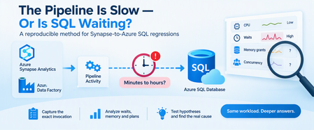
2 TopicsThe Pipeline Is Slow, or Is SQL Waiting? Diagnosing Synapse-to-Azure SQL Regressions
A query can consume very little CPU and still keep a pipeline waiting for hours. A pipeline activity that normally finishes in minutes suddenly starts taking hours. Nothing obvious has changed: The pipeline definition looks the same. The stored procedure looks the same. Azure SQL Database isn't showing sustained high CPU. Pipeline monitoring still points toward the SQL activity. At this point, saying "SQL is slow" isn't enough. The request may actually be: Executing expensive work. Waiting for memory. Blocked by another transaction. Reading more data than before. Running with a different execution plan. Competing with concurrent pipeline activities. Experiencing different cardinality because of different parameter values. The key is to connect the pipeline invocation to the database execution and determine where elapsed time is really going. 1. Define the Regression Precisely Before troubleshooting SQL, establish what actually changed. Capture: Expected pipeline duration. Observed pipeline duration. Pipeline activity involved. Stored procedure or statement invoked. Exact parameter values. Affected and unaffected executions. Pipeline concurrency. Retry behavior. Connection and command timeout. Deployment or configuration changes. For example: Evidence Baseline Regression Pipeline duration Minutes Much longer Stored procedure Same Same Parameter range A B Concurrent activities Low Higher Azure SQL CPU Normal Normal/moderate SQL wait behavior Unknown To investigate The most important rule is: Don't assume the SQL workload is identical simply because the stored procedure is identical. Different parameters can result in dramatically different: Row counts. Join choices. Memory grants. Sort requirements. Execution plans. Total duration. 2. Preserve the Exact Invocation One of the easiest ways to lose a performance regression is to reproduce it with different parameters. Capture the invocation before testing: Procedure name. Parameter values. Date range. Entity or partition identifier. Batch size. Pipeline run ID. Retry number. Number of parallel activities. Relevant timeout configuration. Then sanitize any business-sensitive values before sharing them outside your organization. The diagnostic principle is simple: Reproduce the same workload before trying to improve the workload. 3. Reproduce Safely Whenever possible, reproduce the issue using: A nonproduction database containing representative data. A controlled production troubleshooting window. The same stored procedure. The same parameter pattern. Comparable concurrency. For a controlled test, SQL execution statistics can help: SET STATISTICS IO ON; SET STATISTICS TIME ON; EXEC dbo.SampleProcedure @StartDate = '2026-01-01', @EndDate = '2026-01-31', @EntityID = 100; SET STATISTICS TIME OFF; SET STATISTICS IO OFF; Replace these synthetic names and values with the sanitized equivalent of the invocation you're investigating. Capture: Elapsed time. CPU time. Logical reads. Physical reads when relevant. Execution plan. Returned row count. The goal isn't simply to reproduce "slow." The goal is to understand why it is slow. 4. First Question: Is SQL Running or Waiting? This distinction changes the entire investigation. During the slow execution, examine the active request. SELECT r.session_id, r.request_id, r.status, r.command, r.start_time, r.cpu_time, r.total_elapsed_time, r.wait_type, r.wait_time, r.last_wait_type, r.wait_resource, r.blocking_session_id, r.reads, r.writes, r.logical_reads, r.row_count FROM sys.dm_exec_requests AS r WHERE r.database_id = DB_ID() ORDER BY r.total_elapsed_time DESC; sys.dm_exec_requests is supported for Azure SQL Database and exposes information about currently executing requests. Pay particular attention to the relationship between: cpu_time and: total_elapsed_time Suppose a request has: Very high elapsed time. Relatively little accumulated CPU time. A significant current wait. That's a strong reason to investigate waiting, rather than immediately treating the problem as insufficient CPU. Conversely: High elapsed time. High accumulated CPU. High logical reads. points more strongly toward expensive execution. 5. Identify Blocking Another request may be preventing the pipeline's SQL request from progressing. Start with: SELECT session_id, status, wait_type, wait_time, wait_resource, blocking_session_id, cpu_time, total_elapsed_time FROM sys.dm_exec_requests WHERE blocking_session_id <> 0 ORDER BY wait_time DESC; Blocking can explain a scenario where: Pipeline duration increases dramatically. Database CPU remains moderate. The SQL activity appears "active" for a long time. Microsoft documents sys.dm_exec_requests as one of the tools for identifying requests suspended on lock-related waits and tracing blocking behavior in Azure SQL Database. Don't confuse: "The SQL call took two hours." with: "SQL executed for two hours." Those statements aren't necessarily equivalent. 6. Look at the SQL That's Actually Running During an active incident, retrieve the request and its current SQL text: SELECT r.session_id, r.status, r.command, r.cpu_time, r.total_elapsed_time, r.wait_type, r.blocking_session_id, r.logical_reads, txt.text AS batch_text FROM sys.dm_exec_requests AS r CROSS APPLY sys.dm_exec_sql_text(r.sql_handle) AS txt WHERE r.database_id = DB_ID() ORDER BY r.total_elapsed_time DESC; sys.dm_exec_sql_text accepts the sql_handle exposed by sys.dm_exec_requests and returns the associated SQL batch text. This helps validate an important cross-service question: Is the database executing the statement we think the pipeline invoked? 7. Investigate Memory Grants Some operations need execution memory before they can proceed efficiently. Common examples include: Sorts. Hash joins. Hash aggregates. Some index operations. sys.dm_exec_query_memory_grants exposes queries that: Requested a memory grant and received one. Requested a memory grant and are still waiting. It is supported for Azure SQL Database. SELECT mg.session_id, mg.request_id, mg.dop, mg.request_time, mg.grant_time, mg.requested_memory_kb, mg.granted_memory_kb, mg.required_memory_kb, mg.used_memory_kb, mg.max_used_memory_kb, mg.query_cost, mg.timeout_sec, mg.resource_semaphore_id FROM sys.dm_exec_query_memory_grants AS mg ORDER BY mg.requested_memory_kb DESC; Interpret the important columns carefully: requested_memory_kb Memory requested by the query. granted_memory_kb Memory actually granted. required_memory_kb Minimum memory required for execution. used_memory_kb Memory currently being used. max_used_memory_kb Maximum used so far. grant_time NULL when the requested grant hasn't yet been granted. Microsoft specifically documents that queries waiting for memory grants appear in this DMV, and that grant_time remains NULL until the grant is provided. 8. Find Waiting Memory Grants During the active regression, focus specifically on requests that haven't received their grants: SELECT mg.session_id, mg.request_id, mg.request_time, mg.grant_time, mg.requested_memory_kb, mg.required_memory_kb, mg.granted_memory_kb, mg.timeout_sec, mg.dop, mg.query_cost FROM sys.dm_exec_query_memory_grants AS mg WHERE mg.grant_time IS NULL ORDER BY mg.request_time; If the affected session repeatedly appears here, you now have meaningful evidence supporting a memory-grant contention hypothesis. But that's still not enough to state: "Memory grants caused the pipeline regression." You should also establish: Whether the waiting session is actually the pipeline request. How long it remained waiting. Whether other statements were consuming large grants. Whether concurrency changed. Whether the execution plan requested unusually large memory. Why the query requested that amount of memory. That last question is particularly important. Memory-grant problems can be downstream symptoms of: Poor cardinality estimates. Large sorts. Large hash joins. Plan changes. Data growth. Parameter sensitivity. Microsoft's memory-grant troubleshooting guidance emphasizes that operations such as sorts and hash operations can require execution-memory reservations and that these grants exist for the lifetime of the query. Memory-grant contention is a diagnostic hypothesis until the evidence supports causality. 9. Pipeline Concurrency Is Database Concurrency This connection is easy to overlook. Suppose one stored-procedure invocation performs acceptably. Now imagine the orchestration layer starts: 2 copies concurrently. 5 copies concurrently. 10 copies concurrently. 20 copies concurrently. Each execution may individually be reasonable. Together, they can compete for: CPU. Workers. Memory grants. Buffer pool resources. I/O. Locks. This means: A pipeline concurrency change is also a database workload change. Even when: SQL code hasn't changed. Database configuration hasn't changed. Stored procedure code hasn't changed. As part of troubleshooting, compare: Single-execution performance. Typical production concurrency. Regression-period concurrency. Temporarily reducing pipeline concurrency can also be a valuable diagnostic experiment, provided the change is safe for the workload. 10. Capture the Live Execution Plan For a request that's still executing, Azure SQL Database supports sys.dm_exec_query_statistics_xml(), which returns Showplan XML containing transient execution statistics for an in-flight request. First identify the target session: SELECT session_id, request_id, status, command, cpu_time, total_elapsed_time, wait_type, logical_reads FROM sys.dm_exec_requests WHERE database_id = DB_ID() ORDER BY total_elapsed_time DESC; Then, for a known session: DECLARE @SessionID smallint = 123; SELECT qsx.session_id, qsx.request_id, qsx.query_plan FROM sys.dm_exec_query_statistics_xml(@SessionID) AS qsx; Replace 123 with the session being investigated. The live plan can help answer: Which operator is consuming time? How many rows are flowing through operators? Are estimates diverging significantly from runtime behavior? Are large joins or sorts involved? Where does execution appear to be spending time? Microsoft describes access to execution-plan runtime information as particularly useful when investigating long-running queries, because the information can be inspected without waiting for the query to finish. Use live-plan collection purposefully, especially on heavily loaded production systems. 11. Compare Historical Behavior in Query Store A live snapshot explains what's happening now. Query Store helps answer: What was happening when the query used to be fast? For example, find queries with multiple retained Query Store plans: SELECT TOP (50) q.query_id, COUNT(DISTINCT p.plan_id) AS plan_count, COUNT(DISTINCT p.query_plan_hash) AS distinct_plan_shapes, MIN(p.first_execution_time) AS first_plan_execution, MAX(p.last_execution_time) AS last_plan_execution FROM sys.query_store_query AS q JOIN sys.query_store_plan AS p ON q.query_id = p.query_id GROUP BY q.query_id HAVING COUNT(DISTINCT p.plan_id) > 1 ORDER BY plan_count DESC; Multiple plans aren't automatically evidence of a problem. Instead, investigate whether plan changes correlate with: Pipeline regressions. Duration changes. CPU changes. Logical-read changes. Memory behavior. Different parameter populations. 12. Compare Runtime Distributions, Not Just Averages Averages can hide regression patterns. Consider: Most executions take 10 seconds. A few take 45 minutes. The average won't fully describe the operational impact. For a known Query Store query_id, compare plans and runtime intervals: DECLARE @QueryID bigint = 123; SELECT p.plan_id, rsi.start_time, rsi.end_time, SUM(rs.count_executions) AS execution_count, CAST(AVG(rs.avg_duration) / 1000.0 AS decimal(18,2)) AS avg_duration_ms, CAST(MAX(rs.max_duration) / 1000.0 AS decimal(18,2)) AS max_duration_ms, CAST(AVG(rs.avg_cpu_time) / 1000.0 AS decimal(18,2)) AS avg_cpu_ms, CAST(AVG(rs.avg_logical_io_reads) AS decimal(18,2)) AS avg_logical_reads FROM sys.query_store_query AS q JOIN sys.query_store_plan AS p ON q.query_id = p.query_id JOIN sys.query_store_runtime_stats AS rs ON p.plan_id = rs.plan_id JOIN sys.query_store_runtime_stats_interval AS rsi ON rs.runtime_stats_interval_id = rsi.runtime_stats_interval_id WHERE q.query_id = @QueryID GROUP BY p.plan_id, rsi.start_time, rsi.end_time ORDER BY rsi.start_time DESC, p.plan_id; Replace 123 with the Query Store ID being investigated. Compare: Fast periods. Slow periods. Plans. Execution counts. CPU. Duration. Logical reads. This often produces a better picture than looking at lifetime averages. 13. Don't Force the Fastest Historical Plan Yet Suppose Query Store shows: Plan A took 30 seconds. Plan B takes 20 minutes. It might be tempting to immediately force Plan A. But first ask: How many times did Plan A execute? Which parameters used Plan A? Was the data distribution comparable? Was workload concurrency comparable? Did Plan A perform well repeatedly? Is the query parameter sensitive? A plan that was excellent for one parameter combination might be disastrous for another. The goal isn't to find the lowest historical duration. The goal is to find the plan behavior that's safe for the intended workload. If plan forcing is tested, define rollback criteria before deployment. 14. Test One Hypothesis at a Time Avoid simultaneously changing: Statistics. Indexes. Query code. Pipeline concurrency. Plan forcing. Compute tier. Doing everything together may improve performance, but you'll learn very little about why. Instead: Hypothesis: stale or inaccurate statistics Test: Appropriate statistics maintenance. Same parameters. Same concurrency. Then measure again. Hypothesis: memory-grant contention Test safely with: Reduced concurrency. Same parameter set. Same procedure. Same database configuration. Then compare: Grant wait behavior. Elapsed time. CPU time. Query plan. Hypothesis: plan regression Compare: Historical plans. Representative parameters. Runtime distributions. Only then evaluate targeted plan intervention. Hypothesis: poor cardinality Look for: Estimate-to-actual row differences. Parameter sensitivity. Implicit conversions. Sort/hash behavior. Excessive memory requests. This approach turns troubleshooting from guesswork into experimentation. 15. Correlation Is Not Root Cause This is perhaps the most important principle in cross-service troubleshooting. Suppose you see: A slow pipeline. A SQL memory-grant wait. Several concurrent activities. Those facts are correlated. They don't yet prove: "Memory contention caused the pipeline regression." A stronger conclusion requires a causal chain such as: The pipeline invokes the identified SQL request. That request repeatedly waits for execution memory during the regression. Competing queries hold substantial memory grants during the same period. Reducing the competing concurrency removes or materially reduces the grant wait. The same SQL invocation then returns toward its normal runtime. Repeating the workload reproduces the relationship. Now the evidence for causality is much stronger. This distinction matters because Azure SQL memory pressure can arise from several sources, including the chosen service objective, aggregate workload demand, and individual query memory demand. 16. Build a Cross-Service Evidence Package For difficult Synapse or Data Factory to Azure SQL regressions, both teams should be able to work from the same timeline. Capture: Pipeline evidence Pipeline run ID. Activity name. Activity start and end times. Sanitized parameters. Retry count. Timeout. Concurrent activities. Azure SQL evidence Session/request identification when captured live. Query Store query_id. Query Store plan_id. Runtime intervals. CPU time. Elapsed time. Logical reads. Wait type. Blocking session. Memory grant information. Execution plan. Investigation evidence Separate everything into: Facts Pipeline execution took longer than baseline. SQL request was identified. Request waited for memory. Multiple pipeline activities overlapped. A different plan appeared during the regression. Hypotheses Pipeline concurrency created memory-grant contention. Cardinality changes increased the requested memory grant. Parameter sensitivity caused a plan regression. Blocking contributed to runtime. Resource contention amplified an otherwise acceptable query. Experiments Document: What changed. Why it changed. Test duration. Result. Whether the hypothesis was strengthened or weakened. This prevents the pipeline and database teams from investigating two different incidents that simply happened at the same time. A Practical Decision Tree When a Synapse or Data Factory pipeline's Azure SQL activity suddenly becomes slow: 1. Can you identify the exact invocation? No Capture it before continuing. Yes Reproduce with equivalent parameters and concurrency. 2. Is SQL consuming significant CPU? Yes Investigate: Execution plan. Logical reads. Cardinality. Indexing. Parameter sensitivity. No Look at waits. 3. Is the request blocked? Yes Investigate: Blocking session. Transaction duration. Locking pattern. No Continue. 4. Is the request waiting for a memory grant? Yes Investigate: Requested versus granted memory. Other active grants. Sorts and hash operations. Cardinality estimates. Pipeline concurrency. No Investigate the actual current wait. 5. Did the execution plan change? Yes Compare: Runtime distributions. Parameter sets. CPU. Reads. Memory requirements. No Continue correlating waits, workload volume, and concurrency. 6. Does reducing concurrency improve the same invocation? Yes Resource competition becomes a stronger hypothesis. No Continue investigating query-specific behavior. Final Takeaway When a pipeline goes from minutes to hours, the fact that the Azure SQL activity is taking a long time doesn't automatically mean Azure SQL is spending all that time executing. The request might be spending much of its lifetime: Waiting for memory. Waiting behind another transaction. Waiting for another resource. Executing with a different plan. Processing a different parameter population. Competing with concurrent pipeline activities. A reliable investigation connects two perspectives: Pipeline context What exactly was invoked? With which parameters? At what time? At what concurrency? Database context Was the SQL request executing or waiting? How much CPU did it actually consume? What was it waiting for? Which plan did it use? How much memory did it request? What else was happening concurrently? sys.dm_exec_requests can identify active requests and their current execution state, while sys.dm_exec_query_memory_grants exposes statements that have requested or received execution memory. Azure SQL Database also supports obtaining transient plan information for in-flight requests through sys.dm_exec_query_statistics_xml(). Most importantly: Treat waits, memory grants, plan changes, and concurrency as evidence to test, not automatic root causes. That is how "the pipeline is slow" becomes a reproducible, evidence-backed performance diagnosis.134Views0likes0CommentsLessons Learned #561: It is Fast on the Other Server —What Should We Compare First?
While working on a support case, our customer told us that a stored procedure was taking longer than expected. “It’s fast on the other server,” they explained. Our customer was executing the same stored procedure with the same parameter value in both environments. They had already compared the data and indexes and had not found an obvious explanation for the difference. At that point, we had a symptom, but we still needed evidence to explain it. My first question was simple: was the slower execution doing more work, or taking longer to do comparable work? To answer that question, we needed to look beyond the query text. We would compare the actual execution plans, logical reads, CPU time, and elapsed time, using each observation to guide the next step. In this article, I would like to share how I investigated the problem, step by step. For the demonstration, I will use two tables with identical data and equivalent indexes in the same Azure SQL Database. You can also run this example on two different servers, using one copy of the table on each server. Step 1: Collect evidence from both executions The customer had already compared the data and indexes. Before making any changes, I asked them to collect the same information from both environments: The actual execution plan. The output from SET STATISTICS IO ON. The output from SET STATISTICS TIME ON. We also needed to confirm that both tests used the same parameter value and returned the same results. The execution time told us that there was a difference. These additional details would help us understand why. Logical reads show how many page accesses an execution performs. CPU time shows how much processor time it uses, while elapsed time shows how long it takes. The actual execution plans help us connect those measurements to the operations performed. I wanted to compare this evidence before updating statistics, changing indexes, or recompiling the procedure. Those changes could alter the behavior we were trying to understand. Step 2: The slower execution was doing more work Once we had collected the execution plans and measurements, I started by comparing logical reads, CPU time, and elapsed time. The measurements showed a clear difference: Metric Execution A Execution B Logical reads 30,418 1,532,129 CPU time 219 ms 954 ms Elapsed time 216 ms 1,284 ms Physical reads 0 0 In this sample, execution B took almost six times as long and performed approximately 50 times as many logical reads. We now had an important clue: the slower execution was doing considerably more work. Both executions reported zero physical reads. However, that did not mean that accessing the data was free. Logical reads still represent page accesses through the buffer pool, and repeatedly accessing those pages consumes resources. The higher CPU time in B supported the same observation. Waiting could also contribute to its elapsed time, but waiting alone would not explain the additional logical reads. My next step was to inspect the actual execution plans: which operations were responsible for that extra work? Step 3: An Index Seek does not always mean less work The difference in logical reads gave us a direction. I opened both actual execution plans to see how each execution accessed the data. Execution A used a Clustered Index Scan. It read one million rows, selected the 500,000 that matched the customer, and calculated the total. Execution B used an Index Seek, followed by Nested Loops and a Key Lookup. At first glance, the seek might look like the better choice. It located the customer's orders through the nonclustered index. However, that index did not contain Amount, which the query needed to calculate the total. For each matching order, the plan retrieved the missing value from the clustered index. The Key Lookup executed 500,000 times. That helped explain the additional logical reads: execution B repeatedly accessed the clustered index to retrieve individual rows. Observation Execution A Execution B Access pattern Clustered Index Scan Index Seek followed by Key Lookups Estimated matching rows 500,000 100 Actual matching rows 500,000 500,000 Key Lookup executions None 500,000 The estimates provided our next clue. Execution A expected 500,000 matching rows and received 500,000. Execution B expected only 100, but received 500,000—5,000 times its estimate. A seek followed by a small number of lookups can be efficient. However, repeating those lookups half a million times can become expensive. The plans also used different execution modes: A used batch mode, while B used row mode. This was another difference to keep in mind when comparing CPU and duration. The question was no longer simply why B was slower. Why did its cached plan expect only 100 rows? Step 4: Same runtime parameter, different compiled values To understand the estimate of 100 rows, I checked the parameter information in both actual execution plans. We had executed both procedures with @CustomerId = 2. However, the plans showed an important difference: Parameter property Execution A Execution B ParameterCompiledValue 2 1 ParameterRuntimeValue 2 2 The XML made this easy to see. Execution A: <ColumnReference Column="@CustomerId" ParameterDataType="int" ParameterCompiledValue="(2)" ParameterRuntimeValue="(2)" /> Execution B: <ColumnReference Column="@CustomerId" ParameterDataType="int" ParameterCompiledValue="(1)" ParameterRuntimeValue="(2)" /> ParameterCompiledValue shows the value used when the plan was compiled. ParameterRuntimeValue shows the value used for the execution we captured. Both executions used customer 2, but their plans had been compiled for different customers. Both plans also reported that they were retrieved from cache. In our example, customer 1 has 100 orders, while customer 2 has 500,000. The estimate in B now made sense: its plan had been compiled for the customer with only 100 orders. Using a parameter value during compilation is normal behavior, commonly called parameter sniffing. It helps the optimizer use the available statistics to estimate how many rows the query will process. The difficulty appears when a plan suitable for one parameter value is reused for another value with very different needs. Here, the plan compiled for 100 orders was reused to process 500,000. Different compiled and runtime values alone do not prove a performance problem. In this investigation, however, they connected several observations: the estimate of 100 rows, the 500,000 actual rows, the repeated Key Lookups, and the additional logical reads. We had a strong explanation. Our next step was to test it by compiling for the current parameter and comparing the work again. Step 5: Test the explanation The parameter information gave us a strong clue, but I wanted to test whether a new plan compiled for the current customer would reduce the work. We executed procedure B with the same parameter, this time requesting recompilation: EXEC dbo.GetCustomerOrdersB @CustomerId = 2 WITH RECOMPILE; The new actual execution plan showed both the compiled and runtime parameter values as 2. Instead of the Index Seek followed by 500,000 Key Lookups, the optimizer selected a Clustered Index Scan. It estimated 500,000 matching rows and received 500,000. The measurements also changed: Metric B: original cached plan B: recompiled execution Logical reads 1,532,129 30,418 CPU time 954 ms 344 ms Statement elapsed time 1,284 ms 346 ms Estimated matching rows 100 500,000 Actual matching rows 500,000 500,000 These timings are individual observations, rather than benchmark averages. However, the reduction in logical reads clearly showed that the new execution performed less work. We had not changed the data, added an index, or updated statistics between these executions. The plan XML referenced the same statistics object with the same last-update timestamp and zero modifications. The important change was the plan compiled for the current parameter. It also used batch mode instead of the original plan's row mode. This supported our explanation: the original cached plan was suitable for a customer with few orders, but its repeated lookups became expensive when reused for a customer with 500,000 orders. Recompilation was useful here as a diagnostic test. However, recompiling every execution is not always the best long-term solution. We also need to consider how often the query runs, the cost of compilation, and the parameter values used by the application. What if the query is slower on another server? In this example, the execution history helped explain why equivalent queries performed different amounts of work. In a comparison between two servers, this is one possible cause, but it is not the only one. I would start with the same evidence: actual execution plans, logical reads, CPU time, and elapsed time. From there, we can decide whether to investigate different plans, waits, configuration, or other differences between the environments. For a broader troubleshooting approach, see Microsoft's guide: Troubleshoot a query that shows a significant performance difference between two servers. Can Azure SQL Database handle different parameter needs? Recompilation helped us test our explanation. But could the database use different plans for customers with different numbers of orders, without compiling the query on every execution? This is where Parameter Sensitive Plan optimization, or PSP, can help. For eligible queries, PSP can maintain multiple plan variants and select a variant according to the runtime parameter value. A customer with few orders and a customer with many orders can therefore use different plans for the same parameterized query. PSP is available in Azure SQL Database with compatibility level 160 or later, provided the feature is enabled. Eligibility still matters: enabling it does not guarantee that every query will receive multiple variants. See Parameter Sensitive Plan optimization for details. Our first test deliberately used compatibility level 150. Next, we will repeat the experiment with PSP enabled, keeping the data, indexes, and stored procedures unchanged. We will check both the measurements and the plans to see whether PSP actually intervenes. Step 6: Verify that the feature actually intervenes Next, I repeated the test at compatibility level 160, after enabling PSP in the laboratory database. We executed the procedure for the customer with 100 orders first, followed by the customer with 500,000 orders. The captured plans showed that both executions still used the same plan, compiled for customer 1. The second execution performed 500,000 Key Lookups and reported 1,532,129 logical reads. I also checked the XML for evidence of PSP variants. The captured plans did not contain a dispatcher or a query variant identifier. PSP was enabled, but the captured plans showed no evidence that it was being used. I needed to find out why it had not generated plan variants for this query. Step 7: Check PSP configuration SELECT DB_NAME() AS DatabaseName, compatibility_level FROM sys.databases WHERE database_id = DB_ID(); SELECT name, value FROM sys.database_scoped_configurations WHERE name IN ( 'PARAMETER_SENSITIVE_PLAN_OPTIMIZATION', 'PARAMETER_SNIFFING' ); The results confirmed the configuration/settings: Compatibility level: 160. PARAMETER_SNIFFING: 1. PARAMETER_SENSITIVE_PLAN_OPTIMIZATION: 1. The configuration was correct, so I used Extended Events to find out why PSP had been skipped. I captured the reason during a new compilation using an in-memory ring buffer. -- 1. Create the session DECLARE @sql nvarchar(max); SET @sql = N' CREATE EVENT SESSION Lab_PSP_Reason ON DATABASE ADD EVENT sqlserver.parameter_sensitive_plan_optimization_skipped_reason ( ACTION(sqlserver.sql_text, sqlserver.session_id) WHERE ([sqlserver].[session_id] = (' + CONVERT(nvarchar(12), @@SPID) + N')) ), ADD EVENT sqlserver.query_with_parameter_sensitivity ( ACTION(sqlserver.sql_text, sqlserver.session_id) WHERE ([sqlserver].[session_id] = (' + CONVERT(nvarchar(12), @@SPID) + N')) ) ADD TARGET package0.ring_buffer ( SET max_memory = 1024 ) WITH (MAX_DISPATCH_LATENCY = 1 SECONDS);'; EXEC sys.sp_executesql @sql; ALTER EVENT SESSION Lab_PSP_Reason ON DATABASE STATE = START; -- 2. Trigger a new compilation EXEC sys.sp_recompile N'dbo.GetCustomerOrdersB'; EXEC dbo.GetCustomerOrdersB @CustomerId = 1; EXEC dbo.GetCustomerOrdersB @CustomerId = 2; WAITFOR DELAY '00:00:02'; -- 3. Read the XML before stopping the session SELECT CAST(t.target_data AS xml) AS CapturedEvents FROM sys.dm_xe_database_session_targets AS t JOIN sys.dm_xe_database_sessions AS s ON s.address = t.event_session_address WHERE s.name = N'Lab_PSP_Reason' AND t.target_name = N'ring_buffer'; -- 4. Stop and delete the session ALTER EVENT SESSION Lab_PSP_Reason ON DATABASE STATE = STOP; DROP EVENT SESSION Lab_PSP_Reason ON DATABASE; Why did PSP not generate variants? The database was using compatibility level 160, and both PSP and parameter sniffing were enabled. However, the captured plans still showed the same plan being reused. To understand why, I captured the Extended Event parameter_sensitive_plan_optimization_skipped_reason during a new compilation. It reported: <data name="reason"> <value>30</value> <text>SkewnessThresholdNotMet</text> </data> For this compilation, the optimizer's skewness threshold for PSP was not met, so it did not generate plan variants. This did not mean that the original plan was efficient for both customers. Our earlier measurements had already shown the additional work caused by reusing it for the larger customer. That was another useful lesson from the investigation: check whether an optimization actually intervened, rather than assuming that enabling it resolved the problem. PSP can help eligible queries, but we still need to inspect their plans and measure their behavior. Step 8: Reduce the work behind the slow execution Recompilation had helped us validate the explanation. Next, I wanted to test a change that would reduce the work even when the plan was compiled for the smaller customer. The nonclustered index contained CustomerId, but the query also needed Amount. The original plan retrieved that missing value through a Key Lookup for every matching order. We extended the existing index to include Amount: CREATE NONCLUSTERED INDEX IX_Orders_CustomerId ON dbo.OrdersB (CustomerId) INCLUDE (Amount) WITH (DROP_EXISTING = ON); Then we repeated the sequence that had exposed the problem: compile for the customer with 100 orders, followed by executions for the customer with 500,000 orders. This time, we did not use WITH RECOMPILE for those executions. Metric for the larger customer Before the index change After: first execution After: second execution Logical reads 1,532,129 1,426 1,426 CPU time 984 ms 141 ms 156 ms Elapsed time 1,501 ms 144 ms 154 ms Key Lookup executions 500,000 0 0 These measurements were collected at compatibility level 160 before and after the index change. The new plan obtained the required values directly from the nonclustered index. It no longer needed to retrieve Amount separately from the clustered index for each order. An important detail remained: the plan was still compiled for customer 1 and reused for customer 2. It still estimated 100 matching rows and processed 500,000. We had not eliminated the estimation difference. We had removed the repeated lookups that made that difference expensive in this example. The improvement also did not depend on PSP generating variants: the captured executions reused the same ordinary cached plan. For this query and the tested parameter values, extending the index provided a more efficient access path. Before applying the same approach in production, we would also evaluate the additional index storage and the maintenance cost for data changes. The goal was to reduce the work that made the reused plan expensive. The actual plan and measurements showed that the change achieved that in our test. What I learned from this investigation “It’s fast on the other server” was the starting point. To investigate it, we needed to compare what happened during each execution. In our demonstration, equivalent data and indexes did not lead to equivalent execution plans. Both measured executions used the same parameter, but their cached plans had been compiled for different customers. The slower execution expected 100 matching rows and processed 500,000. Its repeated Key Lookups helped explain the additional logical reads and CPU consumption. Recompilation helped us test that explanation. We then extended the existing index to include Amount, allowing the query to retrieve the required values without those lookups. Even after the index change, the execution for the larger customer reused a plan compiled for the smaller customer. The estimate remained inaccurate for the larger customer, but the expensive lookups were gone. Logical reads dropped from 1,532,129 to 1,426 in our compatibility-level-160 test. We also verified PSP rather than assuming it would intervene. Although it was enabled, Extended Events reported SkewnessThresholdNotMet for the compilation we captured. For me, the practical lessons were: Compare logical reads and CPU alongside elapsed time. Inspect the actual work behind an Index Seek or Scan. Compare estimated and actual rows at the relevant operators. Check compiled and runtime parameter values. Validate a proposed improvement using the execution sequence that exposed the problem. Confirm whether an optimization feature actually participated. The index change addressed the additional work in this example. Other queries may need a different approach, and index changes should be evaluated against the wider workload. When a customer says, “It’s fast on the other server,” my next question is: “What do the two executions show us?” Further reading For a broader investigation of performance differences between servers, see Troubleshoot a query that shows a significant performance difference between two servers. For details about plan variants, eligibility, and diagnostic events, see Parameter Sensitive Plan optimization.353Views0likes0Comments