microsoft fabric
98 Topics
Amplify Healthcare Intelligence: Data, AI, and Agent-Powered Transformation
Join Microsoft for Amplify Healthcare Intelligence, a webinar and in-person workshop series designed for healthcare and life sciences organizations building the foundation for trusted AI. Every session starts from the same premise: you cannot deliver trusted AI without a trusted data foundation. Across the series you will see how leading organizations unify their data estate, ground AI agents in real business context, and turn that foundation into results they can measure. What You Will Learn How to build a unified, AI-ready data foundation across a fragmented healthcare data estate How to ground AI agents in trusted healthcare data and real business context How to modernize analytics while reducing complexity and cost How to accelerate innovation with Microsoft Fabric, Azure AI Foundry, Microsoft IQ, and Copilot technologies How to deliver measurable impact across clinical, operational, research, and business scenarios Whether you are defining your AI strategy, modernizing your analytics platform, or scaling AI across your organization, these sessions offer practical guidance, real-world customer examples, and hands-on learning to help you move from AI ambition to business impact. Webinars & In-Person Workshops 🎥 Webinars One-hour virtual sessions with actionable guidance, live demonstrations, customer stories, and best practices from Microsoft experts. Each webinar shows how leading healthcare organizations are turning data, AI, and enterprise intelligence into measurable business outcomes. All sessions are from 3-4 ET (12-1 PT) and are free to attend. Date Topic Register Oct 21 3-4 ET (12-1 PT) Finance in the Agent Era: AI-Powered Planning, Forecasting, and Insights Register Oct 28 3-4 ET (12-1 PT) Reduce BI Sprawl, Cut Cost and Build an AI-Ready Analytics Foundation Register Cannot join live? Register anyway. We will send you the recording and session materials after the event. Additional sessions will be added through the end of the year, so check back or register for one session to be notified as new dates are announced. 🏢 In-Person Workshops Our two-day workshops combine executive strategy, healthcare-specific use cases, architecture guidance, and hands-on labs designed to help teams identify and accelerate high-value AI opportunities. Attendance is free. Participants are responsible for their own travel and accommodation, and space at each location is limited. Workshops run 9am to 4pm local time on both days. Day 1: From Healthcare Data to Healthcare Intelligence Day 1 focuses on healthcare transformation strategy, customer examples, and the architectural patterns that make trusted AI possible at scale. The day closes with a networking reception and peer exchange. The Frontier Transformation imperative: from AI ambition to measurable impact Microsoft IQ: turning data into enterprise intelligence Building the unified data foundation Building trusted AI: security, governance, privacy, and compliance Healthcare transformation in action: clinical, operational, research, and finance scenarios Activating data with AI data agents and Copilot experiences Day 2: Hands-On Healthcare AI and Analytics Lab Day 2 is a guided, end-to-end lab. Participants build a working healthcare intelligence solution from raw data through to a grounded AI agent, using Microsoft Fabric, Azure AI Foundry, Copilot technologies, and modern data architectures. Build the foundation: data ingestion, lakehouse architecture, and data engineering Create actionable insights: semantic models and dashboards Prepare data for AI: AI-ready data assets and data governance Build and ground AI agents in trusted enterprise data From insight to intelligent action: planning your organization's next steps What to bring: a laptop with a current browser. Lab environments and credentials are provided on site, and no prior Fabric or Foundry experience is assumed. Date City Venue Register November 10-11, 2026 9am - 4pm Chicago Microsoft Chicago (AON Center) 200 East Randolph Drive, Suite 200 Chicago, IL 60601 Register December 8-9, 2026 9am - 4pm New York Microsoft Garage 300 Lafayette Street New York, NY 10012 Register Who Should Attend This series is built for the people who own the data estate and the people who depend on it. Sessions are technical enough for practitioners and strategic enough for the leaders who prioritize the work. Data & analytics leaders Data platform, data engineering, and business intelligence teams Data architects, engineers, and data scientists AI and innovation leaders Healthcare and life sciences executives Clinical, operational, research, and finance transformation leaders No prior Microsoft Fabric or AI experience is required for any session in this series. Questions Contact Camille Whicker if you have any questions about our upcoming events.Tableau to Power BI Migration: Semantic Layer-First Approach for Cloud Architects
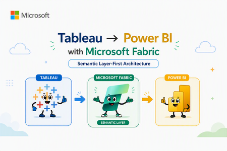
Author's: Mahjabin Ahmed, Yassine El Ouardi, Lavanya Sreedhar LavanyaSreedhar, Peter Lo PeterLo, Aryan Anmol aryananmol, Shreya Harvu shreyaharvu and Rafia Aqil Rafia_Aqil In this guide, we provide practical guidance for migrating from Tableau to Power BI, with a focus on technical best practices and architecture. Unifying business intelligence on the Microsoft Fabric platform, enterprises gain closer integration with Microsoft 365 (Teams, Copilot, Excel). For cloud solution architects and BI developers, a successful migration is not just about rebuilding dashboards in a new tool. It requires thoughtful architectural planning and a shift to a more model-centric approach to BI. Why Semantic Layer-First Architecture Matters The Traditional Migration Challenge Most Tableau to Power BI migrations follow a dashboard-centric approach: teams attempt to replicate existing Tableau workbooks, calculated fields, and LOD (Level of Detail) expressions directly into Power BI reports. While this may seem efficient initially, it creates significant downstream challenges: Duplicated logic: Each report embeds its own calculations and business rules, leading to conflicting KPIs across the organization Maintenance overhead: Changes to business logic require updating dozens or hundreds of individual reports Governance gaps: Without centralized definitions, semantic drift occurs—different teams calculate "Revenue" or "Active Customer" differently Scalability issues: As data volumes grow, report-level transformations become performance bottlenecks The Semantic Layer-First Alternative Microsoft's recommended approach centers on semantic models (formerly called datasets)—centralized, governed data models that separate business logic from visualization. In this architecture: The payoff is substantial: when data evolves or business rules change, you update the semantic model once, and all dependent reports automatically reflect the changes—no manual redesign required. Understanding Migration Complexity: Simple to Very Complex Dashboards Not all Tableau dashboards are created equal. The migration strategy should align with dashboard complexity, and the semantic layer approach becomes increasingly valuable as complexity grows. Follow a Step-by-Step Migration Strategy Migrating from Tableau to Power BI is not a one-click effort – it requires a mix of automated and manual refactoring, plus a sound change management plan. Below are key strategies and best practices for a successful migration: Audit your Tableau estate: Start by taking inventory of all existing Tableau workbooks, data sources, and dashboards. Determine what needs to be migrated (focus on high-value, widely used reports first) and identify any redundant or obsolete content that can be retired rather than converted. Conduct a proof-of-concept (PoC): Before migrating everything, pick a representative complex dashboard (or a subset of your data) and perform a pilot migration. This will help you validate that Power BI can connect to your data (e.g. setting up the Power BI gateways for on-premises sources), test performance (Import vs DirectQuery modes), and experiment with replicating key visuals or calculations. Use the PoC to uncover any surprises early – for example, test that any Level of Detail expressions or table calculations in Tableau can be re-created in DAX. The lessons learned here should inform your overall project plan. Use a phased migration approach: Plan to run Tableau and Power BI in parallel for some period, rather than switching everything at once. Migrate in waves – for example, by business unit or subject area – and incorporate user feedback as you go. This phased approach reduces risk and allows your team to improve the process with each iteration. It also gives end users time to adjust gradually. Migrate high-impact dashboards first: Prioritize the migration of key reports and dashboards that are critical to the business or have the most usage. Delivering these early wins will not only surface any technical challenges to solve but will also help demonstrate the value of Power BI’s capabilities to stakeholders. Early success builds buy-in and momentum for the rest of the migration. Reimagine (don’t just replicate) the experience: It’s rarely possible – or desirable – to exactly re-create every Tableau visualization pixel-for-pixel in Power BI. Embrace the opportunity to focus on business questions and improve user experience with Power BI’s features. For example, rather than replicating a complex Tableau workaround, you might implement a cleaner solution in Power BI using native features (like bookmarks, drilldowns, or simpler navigation between pages). Engage business users and subject matter experts during this redesign to ensure the new reports meet their needs. Enable dataset reusability: One major benefit of the Power BI approach is the ability to create shared datasets and dataflows. As you migrate, look for opportunities to create central semantic models (datasets) that can serve multiple reports. For instance, if several Tableau workbooks are all using similar data about sales, you can create one central Sales dataset in Power BI. Report creators across the organization can then build different Power BI reports on that single dataset without duplicating data or logic. This reduces maintenance and promotes a “build once, reuse often” strategy. Provide training and support: Expect a learning curve for teams moving to Power BI – especially those who are very fluent in Tableau. Plan for user upskilling and training programs. Establish a support community or office hours where new users can ask questions and get help. If possible, identify Power BI champions or recruit a Power BI Center of Excellence (COE) team who can guide others. During the transition, ensure there are subject matter experts (SMEs) available to address questions and validate that the new reports are correct. Manage change and expectations: It’s important to communicate why the organization is moving to Power BI (e.g. benefits like deeper integration, lower TCO, better governance) to get buy-in from end users. Some users may be resistant to change, especially if they’ve invested a lot of time in mastering Tableau. Prepare to handle varying responses – emphasize the personal benefits (like improved performance, new capabilities, or career growth with popular skills) to encourage adoption. Also, involve influential business users early and gather their feedback, so they feel ownership in the new solution. Establish governance from Day 1: Don’t wait until after migration to think about governance. Use this chance to set up Power BI governance aligned to best practices. Decide on important aspects such as workspace naming conventions, who can create or publish content, how you’ll monitor usage and costs, and how to manage data access and security (for example, designing a strategy for RLS/OLS/CLS, and deciding when to use per-user datasets vs. organizational semantic models). Good governance will ensure your shiny new Power BI environment doesn’t sprawl into chaos over time. Allow time for adjustment and iteration: Finally, be patient and iterative. Depending on the scale of your organization and the number of Tableau assets, a full migration can take months or even a year or more. Plan realistic transition periods where both systems might coexist. Continuously refine your approach with each wave of migration. Power BI’s frequent update cadence (monthly releases) means new features may emerge even during your project – stay updated, as new capabilities could simplify your migration (for example, the introduction of field parameters or Copilot might let you modernize certain Tableau features more easily). Reimagine (don’t just replicate) the experience (Step 5): Phase 1: Assessment and Planning 1. Audit Your Tableau Estate Inventory all workbooks, data sources, and calculated fields Identify high-traffic dashboards (prioritize for early migration) Categorize by complexity (Simple/Medium/Complex/Very Complex) 2. Design Your Semantic Architecture Map Tableau data sources to Power BI data sources (DirectQuery, Import, or Direct Lake) Plan star schema for fact/dimension tables Identify shared calculations that should live in semantic models vs. report-specific logic 3. Choose Storage Modes Source Type Recommended Mode Rationale Databricks Delta Lake Direct Lake Real-time analytics, no refresh lag Azure SQL Database DirectQuery or Import Based on data volume and refresh SLAs On-Premises SQL Server Import (via Gateway) Network latency considerations Excel/CSV files Import Small reference data Phase 2: Build the Semantic Layer 1. Create Star Schema Data Models Tableau often relies on flat, denormalized datasets. Power BI performs best with star schemas: Fact tables: Transactional data (sales, orders, events) with foreign keys to dimensions Dimension tables: Descriptive attributes (customers, products, dates) with primary keys Relationships: One-to-many from dimension to fact, leveraging bidirectional filtering sparingly 2. Migrate Calculations to DAX Measures Convert Tableau calculated fields to DAX measures in the semantic model: --Example of DAX: -- Define as measure: Total Revenue = SUMX( 'Sales', 'Sales'[Quantity] * 'Sales'[Unit Price] ) 2.1 Use Copilot to Accelerate DAX Development Leverage Copilot in Power BI Desktop to generate and validate DAX: Describe the calculation in natural language Copilot suggests DAX syntax Review, test, and refine 2.2 Document your Semantic Model Invest in creating an AI-ready foundation for your semantic model. AI systems need to understand unique business contexts in order to prioritize correct information to provide consistent and reliable responses to your end users. Name Tables and Columns Clearly: Avoid ambiguity in your semantic model. Use human-readable, business-friendly names. Avoid abbreviations, acronyms, or technical terms. This improves Copilot’s ability to interpret user intent. Create Meaningful Measures: Define reusable DAX measures for key business metrics (e.g., Revenue, Profit Margin). AI features rely on these to generate insights and summaries. Document Semantic Model objects: Add descriptions and synonyms to your Tables, Columns and measures. This enhances natural language querying and improves Copilot’s contextual understanding. Build an AI Data Schema: prepare your semantic model for AI by utilizing tooling features such as Prep data for AI. Phase 3: Understanding Migration Complexity: Simple to Very Complex Dashboards Not all Tableau dashboards are created equal. The migration strategy should align with dashboard complexity, and the semantic layer approach becomes increasingly valuable as complexity grows. 1. Dashboard Conversion Best Practices Think in "pages" not "sheets": Power BI reports combine multiple visuals per page; group related visuals logically Use slicers for interactivity: Replace Tableau filters with Power BI slicers and filter pane Leverage bookmarks for navigation: Create dynamic report experiences with show/hide containers Simple Complexity Level Category Tableau Feature Power BI Equivalent Microsoft Fabric Enhancements Best Practice Notes Data Model Single custom SQL Power Query for data shaping and ETL. OneLake Shortcuts for unified data access. Use star schema for optimized performance; push logic into the semantic layer rather than visuals. Calculations Basic IF/ELSE, SUM Data Analysis Expressions (DAX) for measures and calculated columns. Copilot for Power BI to assist with DAX creation. Fabric IQ for natural language queries. Centralize calculations in semantic models for consistency and governance. Medium Complexity Level Category Tableau Feature Power BI Equivalent Fabric Enhancements Best Practice Notes Data Model Multiple custom SQL (up to 3) Connect live to databases (Azure Databricks): DirectQuery in Power BI Connect with cloud data sources: Power BI data sources OneLake Shortcuts for unified access without databricks compute cost. Semantic Models can combine multiple sources. Optimize with star schema; Prefer OneLake Shortcuts for performance; avoid heavy transformations in visuals. Calculations Nested IFs, CASE Data Analysis Expressions (DAX) for measures and calculated columns. Copilot for Power BI to assist with DAX creation. Fabric Data Agent for conversational BI. Fabric IQ for natural language queries: Fabric IQ Centralize logic in semantic models; use Copilot for automation and validation; keep calculations reusable. Reporting Tooltip format in Bar and Map visuals Select All/Clear option for Single Select dropdown Standard tooltips offer help tooltips, text, and background formatting. Dynamic tooltip will be able to create the Tooltip page and reuse it in multiple visuals The customization is so much better than the OOB tooltips Create report tooltip pages in Power BI - Power BI | Microsoft Learn Use Clear All Slicers Button. Disable Single Select, Add Clear All Slicers button, Customize the Button and Use the Button Complex Complexity Level Category Tableau Feature Power BI Equivalent Fabric Enhancements Best Practice Notes Data Model Multiple sources Create relationship using more than one column Composite Models in Power BI (DirectQuery + Import) for combining multiple sources, also connect to various cloud services. Dataflows for pre-processing. Power BI allows a relationship between 2 tables based on only one active column. OneLake Shortcuts for unified access without Azure Databricks compute cost; Microsoft Fabric Dataflows Gen2 offers multiple ways to ingest, transform, and load data efficiently. Consolidate sources into semantic models; use Direct Lake for performance; Plan and design data model to comply with star schema supported by Power BI Relationship DAX USERELATIONSHIP DAX for activating relationships in Power BI for a specific calculation Calculations LOD, window functions Data Analysis Expressions (DAX) for measures and calculated columns. Copilot to assist with complex DAX. Fabric IQ Ontology for semantic alignment. Change how visuals interact in a Power BI report. Centralize calculations in semantic layer; use variables in DAX for readability and performance. Fabric Data Agent for a conversational BI. Very Complex Complexity Level Category Tableau Feature Power BI Equivalent Fabric Enhancements Best Practice Notes Data Model Multi-source, Excel, SQL Composite Models in Power BI (DirectQuery + Import) for combining multiple sources, also connect to various cloud services. Dataflows for pre-processing. OneLake Shortcuts for unified access; Connector overview build-in support. Mirroring for real-time sync. Combine multiple sources into well-structured semantic models for consistency and optimized performance. Calculations Predictive logic Data Analysis Expressions (DAX) for measures and calculated columns. Fabric AutoML, ML models, AI Insights, Python/R, Notebook‑based ML (Spark/Scikit‑Learn), Fabric AI Functions, Fabric IQ Ontology Fabric Data Agent for a conversational BI. Centralize logic in semantic models; leverage Copilot for automation and parameter-driven workflows. Prepare for Copilot. 2. Tableau Feature Equivalents Tableau Feature Power BI Equivalent Microsoft Learn Link Calculated Fields DAX Measures DAX Documentation Parameters Field Parameters / Bookmarks Use report readers to change visuals Actions Drillthrough / Bookmarks Drillthrough Tableau Prep Power Query / Dataflows Differences between Dataflow Gen1 and Dataflow Gen2 Tableau Server Power BI Service What is Power BI? Overview of Components and Benefits Phase 4: Governance and Deployment Workspace Planning (Dev / Test / Prod Separation) A proper workspace strategy is essential for governed deployments in Fabric and Power BI. Fabric supports separate Development, Test, and Production stages using Deployment Pipelines, enabling controlled promotions of semantic models, reports, dataflows, notebooks, lakehouses, and other items. You can assign each workspace to a pipeline stage (Dev → Test → Prod) to ensure safe lifecycle management. Sensitivity Labeling (Microsoft Purview Information Protection) Sensitivity labels allow governed classification and protection of data across Fabric items. Sensitivity labels can be applied directly to Fabric items (semantic models, reports, dataflows, etc.) through the item's header flyout or the item settings. Labels from Microsoft Purview Information Protection enforce data access rules and help organizations meet compliance requirements. Endorsement & Certification (Promoted, Certified, Master Data) Endorsement improves discoverability and trust in shared organizational content. Promoted: Item creators mark content as recommended for broader use. Certified: Administrators or authorized reviewers validate content meets organizational quality standards. Master Data: Indicates authoritative single‑source‑of‑truth items such as semantic models or lakehouses. All Fabric items except dashboards can be promoted or certified; data‑containing items can be designated as Master Data. Monitoring & Capacity Planning Determine the appropriate size for fabric capacity when migrating from Tableau to PowerBI. The Fabric SKU Estimator can generate a SKU recommendation (estimate) for your capacity requirements. Ensuring performance and cost efficiency requires ongoing monitoring of your Fabric capacity. Microsoft recommends evaluating workloads using Fabric Capacity Metrics and planning SKU sizes based on real usage. Fabric uses bursting and smoothing to handle spikes while enforcing capacity limits. Monitoring helps identify high compute usage, background refreshes, and interactive workloads to optimize performance. Fabric Data Source Connections (OneLake+ Manage Connections) Microsoft Fabric is designed as an end‑to‑end analytics platform that integrates data from many different source systems into a unified environment powered by OneLake, Data Factory, Real‑Time Analytics, Dataflows , Lakehouses, Warehouses, and Mirrored Databases. The Strategic Advantage: Semantic Layer + Fabric IQ The semantic layer-first approach sets the foundation for the next evolution in enterprise analytics. Fabric IQ (announced at Ignite 2025) is Microsoft's semantic intelligence platform that auto-elevates semantic models into ontologies—structured knowledge graphs that power AI agents, Copilot experiences, and cross-domain data reasoning. What this means for your migration: Semantic models you build today become the foundation for AI-driven analytics tomorrow Data Agents can reason across multiple semantic models, answering questions that span domains Business users transition from "report consumers" to "data explorers" via natural language interfaces Conclusion: Build for the Future, Not Just for Today Migrating from Tableau to Power BI is more than a technology swap—it's an opportunity to re-architect your analytics strategy for the cloud-native, AI-powered era. The semantic layer-first approach requires upfront investment in data modeling, DAX expertise, and Fabric platform adoption. But the payoff is transformative: Consistency: Single source of truth for all business metrics Scalability: Semantic models that serve hundreds of reports and thousands of users Agility: Changes to business logic propagate instantly across the enterprise Future-readiness: Foundation for Fabric IQ, Data Agents, and AI-driven insights Start your migration with the end in mind: not just convert dashboards, but a modern, governed, AI-ready analytics platform that scales with your business. Addressing Key Migration Concerns (1) Why a semantic‑layered model approach is better than recreating Tableau dashboards A semantic‑layered modeling approach is the optimal strategy for migration and is significantly more effective than attempting to recreate Tableau dashboards exactly as they exist. By contrast, Power BI and Fabric encourage a semantic model–first architecture, where all business rules, relationships, calculations, and transformations are centralized in a governed model that serves many dashboards. The approach not only provides consistency and reuse across the enterprise but also ensures that report authors build on a single certified version of the truth. (2) How semantic-layered model approach reduces the constant redesign caused by changing data needs. A semantic‑layered modeling approach directly addresses concern about constant changes and frequent redesigns of dashboards when data evolves. With a semantic layer, changes are absorbed in the model layer—so the logic is updated once and flows automatically into all dependent reports. Combined with Fabric features like OneLake shortcuts, Direct Lake mode, and centralized governance, the semantic layer drastically reduces breakage, minimizes rework, and ensures scalability as data continues to grow and shift. Additional Resources Direct Lake in Microsoft Fabric Create Fabric Data Agents OneLake Shortcuts Write DAX queries with Copilot - DAX Prepare Your Data for AI - Power BI | Microsoft Learn5.1KViews4likes3CommentsOptimizing Oracle-to-Power BI Performance and the Path to Modern Analytics
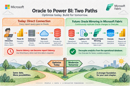
Organizations frequently rely on Oracle databases for large-scale operational workloads while using Microsoft Power BI as their enterprise analytics and visualization platform. Although connecting Power BI directly to Oracle is fully supported, performance can become challenging as datasets grow into the millions of rows. A recent enterprise scenario involving millions of Oracle records illustrates an important principle: Oracle-to-Power BI performance should not be attributed to a single component without first isolating the entire retrieval path. This article provides a practical framework for optimizing that architecture today, while also examining how Microsoft Fabric Mirroring can provide a different data-access pattern for future analytics workloads. The Performance Challenge Consider an Oracle environment containing approximately 15 million records. Testing showed substantially different behavior depending on the client used to retrieve the same Oracle data: A direct Oracle query executed through TOAD returned millions of rows in about eight minutes. Tableau connected to the same Oracle table from the same laptop and refreshed millions of rows in 20 to 30 minutes. Power BI Desktop, however, continued processing for multiple hours before the operation was terminated by network or database controls. Importantly, the Power BI query did not contain additional Power Query transformations. The customer was directly executing SQL and loading the resulting data. This is an extremely useful diagnostic comparison because it demonstrates that Oracle is capable of returning the underlying dataset considerably faster than the Power BI test. It does not, however, prove that the Power BI Oracle connector itself is the single root cause. Performance Is a Pipeline, Not a Single Component Oracle-to-Power BI performance involves several layers: A bottleneck at any one of these layers can affect overall refresh or query performance. Therefore, the first architectural principle is: Measure every layer before attempting to tune the entire solution. A troubleshooting exercise should evaluate: Oracle server-side execution time SQL execution plan Oracle provider/client behavior FetchSize behavior Network transfer Power Query evaluation Query folding Power BI model processing Report design Gateway behavior when the Power BI Service is introduced This approach avoids prematurely concluding that Oracle, Power BI, the gateway, or the connector is inherently responsible for the slowdown. Start With the Oracle Provider Power BI currently provides two important approaches for Oracle connectivity. Built-in Oracle provider Modern versions of Power BI Desktop include Microsoft's bundled Oracle Managed ODP.NET provider. This reduces the dependency on separately installing Oracle client software. For environments using the built-in provider, testing should be performed with a current Power BI Desktop release because provider behavior and defaults can change between releases. Oracle Client for Microsoft Tools Oracle Client for Microsoft Tools, or OCMT, remains another supported option. OCMT configures Oracle Data Provider for .NET and can therefore be tested independently from the built-in provider. This gives architects a useful isolation mechanism: Test A: Built-in Oracle provider vs. Test B: OCMT provider. Use the same: workstation SQL statement Oracle database table credentials network path expected row count Changing several variables simultaneously makes the results considerably harder to interpret. Understand FetchSize One of the most important areas identified during troubleshooting is FetchSize. FetchSize controls how much data the Oracle provider retrieves during each fetch operation. For large datasets, a small FetchSize can require many retrieval operations, increasing overhead. Increasing FetchSize allows the provider to retrieve more data at a time and may improve throughput. However, FetchSize tuning should be tested independently from the choice of Oracle provider. Switching to OCMT, for example, does not by itself demonstrate whether FetchSize tuning improves performance. Benchmark the same SQL and dataset using consistent test conditions and compare elapsed time and throughput. FetchSize controls how much Oracle data the provider pulls back in each retrieval batch. Think of FetchSize like the size of a delivery truck. Imagine Power BI needs to retrieve a very large dataset from Oracle. Small FetchSize: Oracle → 📦 → Power BI Oracle → 📦 → Power BI Oracle → 📦 → Power BI Oracle → 📦 → Power BI ...many retrieval operations Larger FetchSize: Oracle → 📦📦📦📦📦 → Power BI Oracle → 📦📦📦📦📦 → Power BI ...fewer retrieval operations The idea is simple: FetchSize determines how much data the Oracle provider fetches at a time. Examine Oracle Data Types FetchSize is not the only provider consideration. Schema matters. A troubleshooting package should include the table DDL rather than only a list of column names. Pay particular attention to large-object types such as: BLOB CLOB Large-object columns may materially change retrieval behavior and can make simply increasing FetchSize insufficient. Therefore capture: complete table DDL column names Oracle data types row width presence of BLOB/CLOB columns expected total result size Do not optimize FetchSize without understanding the shape of the data being transferred. Filter Rows and Columns as Early as Possible Probably the most universally applicable Power Query optimization is also one of the simplest: Do not retrieve data you do not need. Instead of retrieving every row and column and filtering afterward, reduce the dataset at Oracle whenever possible. Good Oracle SQL should therefore: select only required columns apply restrictive predicates at the source aggregate at Oracle where appropriate avoid unnecessary data transfer This matters substantially when Power BI and Oracle are separated by a network boundary. Preserve Query Folding Power Query query folding allows Power BI transformations to be translated back into SQL executed by the relational source. For relational sources such as Oracle, maintaining folding can substantially reduce the amount of work performed by the Power Query mashup engine. The preferred pattern is: Where practical: filter early remove unnecessary columns early avoid transformations that unexpectedly break folding inspect where folding stops push relational operations back into Oracle For DirectQuery, folding is particularly important because the source remains part of the interactive report-query path. Be Careful With Native SQL and Incremental Refresh Native SQL can be extremely valuable for troubleshooting. Running the same targeted SELECT statement through Power BI that is executed directly against Oracle creates a useful A/B test. It helps isolate questions such as: Is Oracle itself taking a long time? Is Power BI generating a different query? Is additional processing happening after Oracle returns the data? Is the retrieval/provider layer adding significant latency? However, architecture matters. Power BI guidance warns that later Power Query steps cannot necessarily fold after a native SQL query, and native SQL has important implications for incremental refresh. Therefore, native SQL is useful both as an optimization technique in some architectures and as a diagnostic isolation technique, but it should not automatically be substituted for a well-folded Power Query design. Prefer Import for Traditional Oracle BI Workloads If the business does not require near-real-time data, Import should generally be evaluated before DirectQuery for large Oracle analytical workloads. With Import: The latency of Oracle, networking, and the provider is mostly experienced during refresh rather than repeatedly during user interaction. This usually provides a more predictable interactive experience. DirectQuery produces a different dependency chain: As a result, source latency can become report latency. Use DirectQuery when its architectural benefits are required, rather than simply because the source database supports it. Make Incremental Refresh Truly Incremental Import does not necessarily mean repeatedly loading the entire Oracle dataset. For large fact tables, incremental refresh should be evaluated so that only required partitions are refreshed. However, there is an important condition: RangeStart and RangeEnd filtering needs to be pushed back to Oracle. If partition filters do not fold, Power BI can end up retrieving considerably more source data than expected before applying the filtering. Therefore incremental refresh testing should verify that the Oracle query generated by Power BI contains the expected predicates. Treat the Gateway as Its Own Performance Layer Once the workload moves into the Power BI Service, however, the on-premises data gateway becomes another measurable component. For production deployments examine: gateway version Oracle provider/client version CPU memory network proximity to Oracle refresh concurrency DirectQuery concurrency competing workloads Where necessary, large refresh workloads and latency-sensitive DirectQuery workloads can be isolated onto different gateway resources. Do not diagnose gateway performance from a Power BI Desktop test where the gateway is not involved. Optimize DirectQuery If It Cannot Be Avoided Sometimes Import is not viable because users require data with very low latency. If Oracle must remain behind DirectQuery, reduce unnecessary work at every level. At Oracle index frequently filtered columns appropriately review execution plans select only necessary columns reduce returned rows avoid unnecessarily expensive calculations In Power Query maintain query folding push filtering to Oracle minimize transformations requiring local evaluation In the semantic model use efficient dimensional modeling avoid unnecessary high-cardinality columns consider aggregation strategies where appropriate In reports limit visual density use selective filters avoid generating unnecessary simultaneous source queries test with realistic user concurrency DirectQuery performance needs to be assessed as an end-to-end architecture, rather than as an individual SQL benchmark. Collect Diagnostics Before Declaring a Root Cause For difficult Oracle performance cases, establish a repeatable diagnostic package. Capture: Oracle database version execution plan SQL execution duration table DDL data types row count approximate returned data size Provider built-in provider versus OCMT provider/client version FetchSize configuration Power BI Power BI Desktop version generated SQL Query Diagnostics Mashup traces Applied Steps or M code total execution time Network Oracle-to-client path throughput latency connection interruptions or timeouts Comparison clients If Tableau or another Oracle client appears dramatically faster, reproduce the same SQL, same columns, same records, same database and preferably the same machine. Only then does the comparison become a useful engineering benchmark. Future Architecture: Oracle Mirroring in Microsoft Fabric Optimizing the direct Oracle connection solves one class of problem. Microsoft Fabric Mirroring provides a different architecture altogether. Instead of repeatedly placing Oracle in the analytical query path, Fabric can continuously replicate Oracle changes into OneLake. Conceptually: Fabric Mirroring uses Oracle LogMiner to capture changes and maintain an analytical copy in OneLake. This separates many downstream analytical reads from the operational Oracle database. The key architectural advantage isn't simply "a faster connector." The advantage is decoupling analytics from the operational database. Recommended Architecture Decision Tree Requirement: traditional BI with scheduled freshness Use: Oracle → Import → Power BI semantic model. Then optimize: FetchSize provider query folding source-side filtering incremental refresh Requirement: operational or near-real-time reporting where Oracle must remain the source Evaluate: Oracle → DirectQuery → Power BI. But aggressively optimize: Oracle SQL execution plans query folding visual density provider configuration concurrency gateway architecture Requirement: enterprise analytics with frequent Oracle changes and growing BI/AI requirements Evaluate: Oracle → Fabric Mirroring → OneLake → Fabric / Power BI. This reduces repeated analytical pressure against the operational Oracle environment and creates a reusable analytical data foundation for additional workloads. A Practical Troubleshooting Sequence A useful Oracle-to-Power BI performance investigation can be organized into five phases. Phase 1: Establish the Oracle baseline Execute exactly the same query directly against Oracle. Record: SQL → rows → bytes → execution time Phase 2: Isolate the provider Run the same dataset through: Built-in Oracle provider and OCMT. Record the results independently. Phase 3: Test FetchSize Test controlled FetchSize values while holding every other variable constant. Measure throughput rather than relying on subjective impressions. Phase 4: Optimize Power Query Validate: query folding source filtering column projection transformations incremental refresh behavior Phase 5: Decide whether the architecture itself should change If extremely large Oracle datasets must continually feed analytical workloads, consider whether repeatedly querying Oracle remains the appropriate long-term design. At that point, Fabric Mirroring becomes an architectural discussion rather than simply another troubleshooting step. Final Takeaway Oracle-to-Power BI performance problems should not immediately be categorized as an Oracle problem, a Power BI problem, or a gateway problem. They are usually best investigated as a data retrieval pipeline. For existing Power BI architectures, the strongest optimization sequence is: Efficient Oracle SQL For the longer term, Microsoft Fabric Mirroring changes the architecture: Oracle becomes the operational system of record while OneLake becomes the analytical data plane. That separation can be particularly valuable as organizations expand from traditional Power BI reporting into broader Fabric analytics, data engineering and AI workloads.238Views1like0CommentsMGDC for SharePoint FAQ: How to List SharePoint Webs or Subsites?
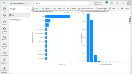
1. Introduction SharePoint uses a known object hierarchy to store your files, including, in order: Site Collection (site, SPSite) Web (site, subsite, SPWeb) List (SPList, Document Library, SPDocumentLibrary) Folder (SPFolder) List Item (documents, files, SPListItem, SPFile) If you are not familiar with all those, you can read more about them at What is in the Permissions dataset? 2.What we have in MGDC for SharePoint The SharePoint Sites dataset in Microsoft Graph Data Connect offers a list of all sites (site collections) in your tenant. The SharePoint Files will give you details about each file (document). However, there are no MGDC datasets that will give you one object per SharePoint Web (subsite) or SharePoint List (library). There is a workaround, though. If you pay attention to the schema for the SharePoint Sites and SharePoint Files datasets in MGDC, you will find that Sites includes a few interesting details about the Root Web (the main web in the site collection) and the total number of webs (subsites) in each site. Also, the Files dataset includes details about the web (subsite) and the list (library) where the file lives. You could group on these columns to expose more information about webs and lists. 3. One Web These days, if you create a modern SharePoint site, you will get one web (called the Root Web) and no obvious mechanism to create subsites or additional webs. For any sites created in the last few years, you likely have no additional webs outside the Root Web. Your SharePoint might have existed for many years and your company could have sites using old templates with multiple subsites. If you’re trying to find out if that’s the case for your tenant, the information is available in MGDC, if you are willing to dig a little deeper. 4. Finding Old Subsites The main task here is to create a custom query to join the Sites and Files datasets. You would then group that in a particular way to enumerate each subsites (Webs). You might also tag the Webs that are a Root Web, so that you can identify subsites that are not at the top of the Site hierarchy. If you pulled the Sites and Files datasets into a SQL Server or a Lakehouse in Microsoft Fabric, this is what that query could look like: SELECT Webs.SiteId, Sites.RootWeb.Title AS SiteTitle, Sites.Url AS SiteUrl, Sites.WebCount, Webs.WebId, CASE WHEN Root.RootWeb.Id IS NOT NULL THEN 1 ELSE 0 END AS IsRootWeb, Webs.FileCount, Webs.TotalSize, Webs.TotalSizeWithVersions FROM ( SELECT SiteId, WebId, COUNT(*) AS FileCount, SUM(SizeInBytes) AS TotalSize, SUM(SizeInBytesWithVersions) AS TotalSizeWithVersions FROM Files GROUP BY SiteId, WebId ) AS Webs LEFT JOIN Sites AS Sites ON Webs.SiteId = Sites.Id LEFT JOIN Sites AS Root ON Webs.SiteId = Root.Id AND Webs.WebId = Root.RootWeb.Id 4. Empty Webs, Web properties This technique will get you a nice list of Webs, but there are a few problems. First, if a specific web has no files, we won’t see that web in the Files dataset and therefore the query will fail to list that particular web. You would still see that Web counted in the WebCount property of the Sites dataset, but there would be no listing of that web in the query proposed above, since it has no files. Another problem is that there is no way to find in MGDC the details properties of the Web, like the Title. You get some of those for the Root Web in the Sites dataset, but not for the other Webs. For that, you would have to query the Web object using another source like the Graph API or PowerShell. 5. Conclusion I hope this article helped you find details about enumerating SharePoint Webs using the Microsoft Graph Data Connect. For recent deployments of SharePoint Online, you should have only one web per site and the Sites dataset (with Root Web details) should give you plenty of details. However, this might come in handy if you want to manage some of the old subsites of a slightly older SharePoint deployment. Finally, if you’re looking for a challenge, I would suggest adapting the SQL code above to enumerate all the document libraries using the Files dataset. It can be done following a similar pattern…Understanding the Notebooks in the Oversharing Template v2 (Microsoft Fabric)
Introduction The Microsoft Graph Data Connect for SharePoint team published two notebooks used with Microsoft Fabric in the Information Oversharing v2 template. This blog explains what each code block inside these notebooks does. The goal was to help you understand what the notebooks do. Note that this document was written with help from Copilot, using simple prompts like “Analyze each section of this Jupyter notebook with PySpark and Scala code. Describe what each section does.” Notebook 1: Read Last Snapshot Dates This first notebook runs right as the pipeline starts. It checks the environment, verifies if the Sites and Permission tables exist in the Lakehouse, checks the last day data was gathered from MGDC and calculates the start and end date to use. It also cleans the staging tables and stores a few commands that are used in later steps. Section 0 – Set the Default Lakehouse for Notebook to Run %%configure { "defaultLakehouse": { "name": { "parameterName": "lakehouseName", "defaultValue": "defaultlakehousename" } } } This section uses the %%configure magic command to set a JSON configuration that defines a parameter (lakehouseName) with the default value "defaultlakehousename". This setting ensures that when the notebook is launched through a pipeline, it dynamically selects the target Lakehouse. Section 1 – Initialize Parameters import java.time.LocalDateTime import java.time.format.DateTimeFormatter import java.time.temporal.ChronoUnit import java.util.UUID import java.text.SimpleDateFormat import java.time.{LocalDate, LocalDateTime, Period} import java.time.format.DateTimeFormatter import java.time.temporal.ChronoUnit import java.util.Calendar import java.sql.Timestamp val runId = "00000000-0000-0000-0000-000000000000" val workspaceId = spark.conf.get("trident.workspace.id") val workspaceName = "LakeHouseTesting" val lakehouseId = spark.conf.get("trident.lakehouse.id") val lakehouseName = "IMAXDefault" val sitesStagingTableName = "Sites_Staging" val sitesFinalTableName = "Sites" val permissionsStagingTableName = "Permissions_Staging" val permissionsFinalTableName = "Permissions" val endTime = "2024-11-15T00:00:00Z" spark.conf.set("spark.sql.caseSensitive", true) This section imports various libraries for date/time handling and initializes key parameters for the ETL process. These include a run identifier (runId), workspace and Lakehouse information (with some values coming from Spark configuration), table names for staging and final datasets, and a fallback endTime. It also enforces case sensitivity in Spark SQL. Section 2 – Checking Required Final Tables Exist or Not val lakehouse = mssparkutils.lakehouse.get(lakehouseName) val lakehouseId = lakehouse.id val workspaceName = notebookutils.runtime.context("currentWorkspaceName") val permissionsStagingLocation = s"abfss://${workspaceName}@onelake.dfs.fabric.microsoft.com/${lakehouseName}.Lakehouse/Tables/${permissionsStagingTableName}" val sitesStagingLocation = s"abfss://${workspaceName}@onelake.dfs.fabric.microsoft.com/${lakehouseName}.Lakehouse/Tables/${sitesStagingTableName}" val sitesFinalLocation = s"abfss://${workspaceName}@onelake.dfs.fabric.microsoft.com/${lakehouseName}.Lakehouse/Tables/${sitesFinalTableName}" val permissionsFinalLocation = s"abfss://${workspaceName}@onelake.dfs.fabric.microsoft.com/${lakehouseName}.Lakehouse/Tables/${permissionsFinalTableName}" val tables = spark.catalog.listTables() val siteTableCount = tables.filter(col("name") === lit(sitesFinalTableName) and array_contains(col("namespace"), lakehouseName) ).count() val permissionsTableCount = tables.filter(col("name") === lit(permissionsFinalTableName) and array_contains(col("namespace"), lakehouseName)).count() val siteStagingTableCount = tables.filter(col("name") === lit(sitesStagingTableName) and array_contains(col("namespace"), lakehouseName) ).count() val permissionsStagingTableCount = tables.filter(col("name") === lit(permissionsStagingTableName) and array_contains(col("namespace"), lakehouseName)).count() This section retrieves the Lakehouse object and uses it to construct ABFS paths for both staging and final tables (for Sites and Permissions). It then checks for the existence of these tables by listing them in Spark’s catalog and filtering by name and namespace. Section 3 – Getting Snapshot Dates from Last Successful Extracts import org.apache.spark.sql.functions.{col, _} import org.apache.spark.sql.types._ import org.apache.spark.sql.{DataFrame, Row, SparkSession} import org.apache.spark.storage.StorageLevel val dtCurrentDateFormatt = DateTimeFormatter.ofPattern("yyyy-MM-dd HH:mm:ss.S") val dtRequiredtDateFormatt = DateTimeFormatter.ofPattern("yyyy-MM-dd'T'HH:mm:ss'Z'") var siteDataExists: Boolean = false var permissionsDataExists: Boolean = false val siteSnapshotDate = { if (siteTableCount == 1) { val dfSites = spark.sql(s"SELECT MAX(SnapshotDate) AS SnapshotDate FROM ${lakehouseName}.${sitesFinalTableName} ") val rowSites: Row = dfSites.select("SnapshotDate").head(1)(0) if (rowSites.get(0) == null) endTime else { siteDataExists = true println(s"Sites data Exists: ${siteDataExists}") LocalDateTime.parse(rowSites.get(0).toString(), dtCurrentDateFormatt) .format(dtRequiredtDateFormatt) } } else { endTime } } val permissionsSnapshotDate = { if (permissionsTableCount == 1) { val dfPermissions = spark.sql(s"SELECT MAX(SnapshotDate) AS SnapshotDate FROM ${lakehouseName}.${permissionsFinalTableName} ") val rowPermissions: Row = dfPermissions.select("SnapshotDate").head(1)(0) if (rowPermissions.get(0) == null) endTime else { permissionsDataExists = true println(s"Permissions data Exists: ${permissionsDataExists}") LocalDateTime.parse(rowPermissions.get(0).toString(), dtCurrentDateFormatt) .format(dtRequiredtDateFormatt) } } else { endTime } } This section queries the final tables to retrieve the latest SnapshotDate for both Sites and Permissions. It then reformats the date into an ISO-compliant format. If no snapshot date is found, it defaults to the predefined endTime, and two boolean flags (siteDataExists and permissionsDataExists) are toggled accordingly. Section 4 – Generate View Script for Sites val sitesView: String = s""" CREATE OR ALTER VIEW vw${sitesFinalTableName} AS SELECT *, [StorageQuotaFriendly] = (case when StorageQuota < 1048576 then concat(ceiling(StorageQuota / 1024.0), ' KB') when StorageQuota < 1073741824 then concat(ceiling(StorageQuota / 1048576.0), ' MB') when StorageQuota < 1099511627776 then concat(ceiling(StorageQuota / 1073741824.0), ' GB') when StorageQuota < 1125899906842624 then concat(ceiling(StorageQuota / 1099511627776.0), ' TB') else concat(ceiling(StorageQuota / 1125899906842624.0), ' PB') end ), [StorageUsedFriendly] = (case when StorageUsed < 1048576 then concat(ceiling(StorageUsed / 1024.0), ' KB') when StorageUsed < 1073741824 then concat(ceiling(StorageUsed / 1048576.0), ' MB') when StorageUsed < 1099511627776 then concat(ceiling(StorageUsed / 1073741824.0), ' GB') when StorageUsed < 1125899906842624 then concat(ceiling(StorageUsed / 1099511627776.0), ' TB') else concat(ceiling(StorageUsed / 1125899906842624.0), ' PB') end ) FROM ${sitesFinalTableName} """.stripMargin.replaceAll("[\n\r]"," ") println(sitesView) Here a SQL view (vwSites) is dynamically generated for the Sites final table. The view adds two computed columns (StorageQuotaFriendly and StorageUsedFriendly) that convert byte values into more digestible units such as KB, MB, GB, etc. This script will be stored and executed later. Section 5 – Generate View Script for Permissions val permissionsView: String = s""" CREATE OR ALTER VIEW vw${permissionsFinalTableName} AS SELECT *, ShareeDomain = CASE WHEN CHARINDEX('@', SharedWith_Email) > 0 AND CHARINDEX('.', SharedWith_Email) > 0 THEN SUBSTRING(SharedWith_Email,CHARINDEX('@', SharedWith_Email)+1,LEN(SharedWith_Email)) ELSE '' END, ShareeEMail = CASE WHEN CHARINDEX('@', SharedWith_Email) > 0 THEN SharedWith_Email ELSE '' END, PermissionsUniqueKey = CONCAT(SiteId,'_',RoleDefinition,'_',ScopeId,'_',COALESCE(LinkId,'00000000-0000-0000-0000-000000000000')), EEEUPermissionsCount = SUM(CASE WHEN SharedWith_Name LIKE 'Everyone except external users' THEN 1 ELSE NULL END ) OVER( PARTITION BY CONCAT(SiteId,'_',RoleDefinition,'_',ScopeId,'_',COALESCE(LinkId,'00000000-0000-0000-0000-000000000000'),SharedWith_Name) ), ExternalUserCount = SUM(CASE WHEN SharedWith_TypeV2 LIKE 'External' THEN 1 ELSE NULL END ) OVER( PARTITION BY CONCAT(SiteId,'_',RoleDefinition,'_',ScopeId,'_',COALESCE(LinkId,'00000000-0000-0000-0000-000000000000'),SharedWith_Name) ), B2BUserCount = SUM(CASE WHEN SharedWith_TypeV2 LIKE 'B2BUser' THEN 1 ELSE NULL END ) OVER( PARTITION BY CONCAT(SiteId,'_',RoleDefinition,'_',ScopeId,'_',COALESCE(LinkId,'00000000-0000-0000-0000-000000000000'),SharedWith_Name) ) FROM ${permissionsFinalTableName} """.stripMargin.replaceAll("[\n\r]"," ") println(permissionsView) This section builds a SQL view (vwPermissions) for the Permissions final table. It derives additional columns like ShareeDomain, ShareeEMail, and a composite key (PermissionsUniqueKey) while applying window functions to compute counts (e.g., for external or B2B users). This script will also be stored and executed later. Section 6 – Truncate the Staging Tables from Previous Runs if (siteStagingTableCount == 1) { spark.sql(s"DELETE FROM ${lakehouseName}.${sitesStagingTableName} ") println(s"Staging table deleted: ${lakehouseName}.${sitesStagingTableName}") } else { println(s"Staging table ${lakehouseName}.${sitesFinalTableName} not found") } if (permissionsStagingTableCount == 1) { spark.sql(s"DELETE FROM ${lakehouseName}.${permissionsStagingTableName} ") println(s"Staging table deleted: ${lakehouseName}.${permissionsStagingTableName}") } else { println(s"Staging table ${lakehouseName}.${permissionsStagingTableName} not found") } This section checks if the staging tables exist (by count) and, if found, issues a SQL DELETE command to remove existing data so that new data can be loaded. It prints messages indicating the action taken. Section 7 – Return Snapshot Dates Back to Pipeline import mssparkutils.notebook val returnData = s"""{\"LakehouseId\": \"${lakehouseId}\", \"SitesStagingTableName\": \"${sitesStagingTableName}\", \"SitesFinalTableName\": \"${sitesFinalTableName}\", \"SitesSnapshotDate\": \"${siteSnapshotDate}\", \"SitesDataExists\": ${siteDataExists}, \"SitesView\": \"${sitesView}\", \"PermissionsStagingTableName\": \"${permissionsStagingTableName}\", \"PermissionsFinalTableName\": \"${permissionsFinalTableName}\", \"PermissionsSnapshotDate\": \"${permissionsSnapshotDate}\", \"EndSnapshotDate\": \"${endTime}\", \"PermissionsDataExists\": ${permissionsDataExists}, \"PermissionsView\": \"${permissionsView}\"}""" println(returnData) mssparkutils.notebook.exit(returnData) This concluding section aggregates the key metadata—including Lakehouse information, table names, snapshot dates, existence flags, and the generated view scripts—into a JSON string. It then exits the notebook by returning that JSON to the pipeline. Notebook 2: Merge Sites and Permissions to Final Table This notebook runs after the Sites and Permissions data from MGDC has been collected successfully into the staging tables. If this is the first collection, it handles them as full datasets, storing the data directly in the final tables. If this is using MGDC for SharePoint delta datasets, it merges the new, updated or deleted objects from the staging tables into the final tables. Note: The word "Delta" here might refer to Delta Parquet (an efficient data storage format used by tables in a Microsoft Fabric Lakehouse) or to the MGDC for SharePoint Delta datasets (how MGDC can return only the objects that are new, updated or deleted between two dates). It can be a bit confusing, so be aware of the two interpretations of the word. Section 0 – Set the Default Lakehouse for Notebook to Run %%configure { "defaultLakehouse": { "name": { "parameterName": "lakehouseName", "defaultValue": "defaultlakehousename" } } } This section uses the same Lakehouse configuration as in Notebook 1. It sets the default Lakehouse through a parameter (lakehouseName) to support dynamic running of the notebook in different environments. Section 1 – Initialize Parameters import java.time.LocalDateTime import java.time.format.DateTimeFormatter import java.time.temporal.ChronoUnit import java.util.UUID import java.text.SimpleDateFormat import java.time.{LocalDate, LocalDateTime, Period} import java.time.format.DateTimeFormatter import java.time.temporal.ChronoUnit import java.util.Calendar val runId = "00000000-0000-0000-0000-000000000000" val workspaceId = spark.conf.get("trident.workspace.id") val workspaceName = "LakeHouseTesting" val lakehouseId = spark.conf.get("trident.lakehouse.id") val lakehouseName = spark.conf.get("trident.lakehouse.name") val sitesStagingTableName = "Sites_Staging" val sitesFinalTableName = "Sites" val permissionsStagingTableName = "Permissions_Staging" val permissionsFinalTableName = "Permissions" spark.conf.set("spark.sql.caseSensitive", true) This section is like Notebook 1’s Section 1 but here lakehouseName is retrieved from the configuration. It initializes variables needed for merging, such as run IDs, workspace/Lakehouse identifiers, and table names. Section 2 – Read Sites Dataset from Staging Table val lakehouse = mssparkutils.lakehouse.get(lakehouseName) val lakehouseId = lakehouse.id val workspaceName = notebookutils.runtime.context("currentWorkspaceName") println("Started reading Sites dataset") val sitesStagingLocation = s"abfss://${workspaceName}@onelake.dfs.fabric.microsoft.com/${lakehouseName}.Lakehouse/Tables/${sitesStagingTableName}" val dfSitesStaging = spark.read.format("delta").load(sitesStagingLocation) println("Completed reading Sites dataset") This section constructs the ABFS path for the Sites staging table and reads the dataset into a DataFrame using the Delta Parquet format. It includes print statements to track progress. Section 3 – Read Permissions Dataset from Staging Table println("Started reading Permissions dataset") val permissionsStagingLocation = s"abfss://${workspaceName}@onelake.dfs.fabric.microsoft.com/${lakehouseName}.Lakehouse/Tables/${permissionsStagingTableName}" val dfPermissionsStaging = spark.read.format("delta").load(permissionsStagingLocation) println("Completed reading Permissions dataset") This section performs the analogous operation for the Permissions staging table, loading the dataset into a DataFrame and providing console output for monitoring. Section 4 – Check Final Tables Exist or Not import io.delta.tables.DeltaTable val sitesFinalLocation = s"abfss://${workspaceName}@onelake.dfs.fabric.microsoft.com/${lakehouseName}.Lakehouse/Tables/${sitesFinalTableName}" val permissionsFinalLocation = s"abfss://${workspaceName}@onelake.dfs.fabric.microsoft.com/${lakehouseName}.Lakehouse/Tables/${permissionsFinalTableName}" val sitesFinalTableExists = DeltaTable.isDeltaTable(spark, sitesFinalLocation) if (!sitesFinalTableExists) { println("Final Sites table not exists. Creating final Sites table with schema only") dfSitesStaging.filter("1=2").write.format("delta").mode("overwrite").save(sitesFinalLocation) println("Final Sites table created") } else { println("Final Sites table exists already") } val permissionsFinalTableExists = DeltaTable.isDeltaTable(spark, permissionsFinalLocation) if (!permissionsFinalTableExists) { println("Final Permissions table not exists. Creating final Permissions table with schema only") dfPermissionsStaging.filter("1=2").write.format("delta").mode("overwrite").save(permissionsFinalLocation) println("Final Permissions table created") } else { println("Final Permissions table exists already") } This section checks whether the final tables for Sites and Permissions exist. If a table does not exist, it creates an empty table (schema only) from the staging DataFrame by filtering out data (filter("1=2")). Section 5 – Merge Sites Data from Staging Table to Final Table import io.delta.tables._ import org.apache.spark.sql.functions._ import org.apache.spark.sql.expressions.{Window, WindowSpec} import org.apache.spark.sql.functions.{coalesce, lit, sum, col, _} import org.apache.spark.sql.types.{StructField, _} import org.apache.spark.sql.{DataFrame, Row, SparkSession} import org.apache.spark.storage.StorageLevel val deltaTableSource = DeltaTable.forPath(spark, sitesStagingLocation) val deltaTableTarget = DeltaTable.forPath(spark, sitesFinalLocation) import spark.implicits._ val dfSource = deltaTableSource.toDF //Delete records that have Operation as Deleted println("Merging Sites dataset from current staging table") deltaTableTarget .as("target") .merge( dfSource.as("source"), "source.Id = target.Id") .whenMatched("source. Operation = 'Deleted'") .delete() .whenMatched("source.Operation != 'Deleted'") .updateAll() .whenNotMatched("source.Operation != 'Deleted'") .insertAll() .execute() println("Merging of Sites dataset completed") This section performs a Delta Lake merge (upsert) operation on the Sites data. The merge logic deletes matching records when the source’s Operation is 'Deleted', updates other matching records, and inserts new records that are not marked as 'Deleted'. Section 6 – Merge Permissions Data from Staging Table to Final Table import io.delta.tables._ import org.apache.spark.sql.functions._ import org.apache.spark.sql.expressions.{Window, WindowSpec} import org.apache.spark.sql.functions.{coalesce, lit, sum, col, _} import org.apache.spark.sql.types.{StructField, _} import org.apache.spark.sql.{DataFrame, Row, SparkSession} import org.apache.spark.storage.StorageLevel val deltaTablePermissionsSource = DeltaTable.forPath(spark, permissionsStagingLocation) val deltaTablePermissionsTarget = DeltaTable.forPath(spark, permissionsFinalLocation) import spark.implicits._ val dfPermissionsSource = deltaTablePermissionsSource.toDF //Delete records that have Operation as Deleted println("Merging Permissions dataset from current staging table") deltaTablePermissionsTarget .as("target") .merge( dfPermissionsSource.as("source"), """source.SiteId = target.SiteId and source.ScopeId = target.ScopeId and source.LinkId = target.LinkId and source.RoleDefinition = target.RoleDefinition and coalesce(source.SharedWith_Name,"") = coalesce(target.SharedWith_Name,"") and coalesce(source.SharedWith_TypeV2,"") = coalesce(target.SharedWith_TypeV2,"") and coalesce(source.SharedWith_Email,"") = coalesce(target.SharedWith_Email,"") and coalesce(source.SharedWith_AADObjectId,"") = coalesce(target.SharedWith_AADObjectId,"") """) .whenMatched("source. Operation = 'Deleted'") .delete() .whenMatched("source.Operation != 'Deleted'") .updateAll() .whenNotMatched("source.Operation != 'Deleted'") .insertAll() .execute() println("Merging of Permissions dataset completed") This section performs a merge operation on the Permissions data. The merge condition is more complex—comparing multiple columns (including handling nulls with coalesce) to identify matching records. The operation applies deletion for rows marked as 'Deleted', updates others, and inserts records where no match exists. Section 7 – Read and Display Sample TOP 10 Rows var sqlQuery = s"SELECT * FROM ${lakehouseName}.${sitesFinalTableName} order by SnapshotDate DESC LIMIT 10" val dfSitesAll = spark.sql(sqlQuery) display(dfSitesAll) sqlQuery = s"SELECT * FROM ${lakehouseName}.${permissionsFinalTableName} order by SnapshotDate DESC LIMIT 10" val dfPermissionsAll = spark.sql(sqlQuery) display(dfPermissionsAll) This final section executes SQL queries to retrieve and display the top 10 rows from both the Sites and Permissions final tables. The rows are ordered by SnapshotDate in descending order. This is typically used for sample or debugging purposes. Conclusion I hope this article helped you understand the notebooks included in the template. This might help you customize it later. These templates are intended as starting points for your work with many scenarios. Read more about MGDC for SharePoint at https://aka.ms/SharePointData.Information Oversharing v2 Template with Microsoft Fabric
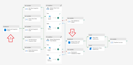
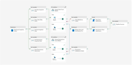
1. Security Scenario One of the most common scenarios for Microsoft Graph Data Connect (MGDC) for SharePoint is Information Oversharing. This security scenario focuses on identifying which items are being widely shared within the tenant and understanding how permissions are applied at each level. The MGDC datasets for this scenario are SharePoint Sites and SharePoint Permissions. If you’re not familiar with these datasets, you can find details in the schema definitions at https://aka.ms/SharePointDatasets. To assist you in using these datasets, the team has developed an Information Oversharing Template. Initially published as a template for Azure Synapse, we now have a new Microsoft Fabric template that is simpler and offers more features. The SharePoint Information Oversharing v2 template, based on Microsoft Fabric, is now publicly available. 2. Instructions The template comes with a set of detailed instructions at https://aka.ms/fabricoversharingtemplatesteps. These instructions include: How to install the Microsoft Fabric and Microsoft Graph Data Connect prerequisites How to import the pipeline template from the Microsoft Fabric gallery and set it up How to import the Power BI template and configure the data source settings See below some additional details about the template. 3. Microsoft Fabric Pipeline After you import the pipeline template, it will look like this: The Information Oversharing template for Microsoft Fabric includes a few key improvements: It uses the new UserCount and TotalUserCount properties in the SharePoint Permissions dataset, which means you do not need to pull the SharePoint Groups or the three Microsoft Entra ID Group datasets to calculate the number of users being granted access. This optimization will greatly reduce the cost to get a report of the sites shared with the most users. The new template also uses delta datasets to update the SharePoint Sites and SharePoint Permissions datasets. It keeps track of the last time the datasets were pulled by this pipeline, requesting just what changed since then. As the previous template, this one also flattens the SharePoint Permissions dataset, creating one permission row for each "Shared With" inside the permission. So, if a file is shared with three people, the SharePoint dataset will show one row, but the flattened data stored in Microsoft Fabric will show three rows. You can find details on how to find and deploy the Microsoft Fabric template in the instructions (see item 3). 4. Microsoft Fabric Report The typical result from this solution is a set of Power BI dashboards pulled from the Microsoft Fabric data source. Here is an example: These dashboards serve as examples or starting points and can be modified as necessary for various visualizations of the data within these datasets. The instructions (see item 3) include details on how to find and deploy a few sample Power BI Information Oversharing templates. 5. Conclusion I hope this provides a good overview of the Information Oversharing template for Microsoft Fabric. You can read more about the Microsoft Graph Data Connect for SharePoint at https://aka.ms/SharePointData. There you will find many details, including a list of datasets available, other common scenarios and frequently asked questions.Streaming and Batch Data Architectures with Microsoft Fabric to Azure Databricks
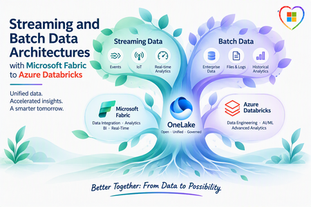
Author's: Aladdin Alchalabi AladdinAlchalabi, Oscar Alvarado oscaralvarado and Rafia Aqil Rafia_Aqil Note: This article describes a solution idea. Your cloud architect can use this guidance to help visualize the major components for a typical implementation. Use this article as a starting point to design a well-architected solution that aligns with your workload’s specific requirements. As organizations adopt Microsoft Fabric as their unified analytics platform, it has become a leading path for ingesting both streaming and batch data into Azure Databricks. This article covers integration approaches -via Microsoft Fabric- and details the five Fabric-specific paths that connect OneLake/ADLS and Databricks for end-to-end data processing. Medallion Architecture The following data flow corresponds to the architecture diagram: Data is ingested through Microsoft Fabric (via Mirroring, RTI, or Data Factory) lands data into OneLake/ADLS. With the medallion pattern, consisting of Bronze, Silver, and Gold storage layers, organizations have flexible access and extendable data processing: Bronze – Raw data entry point. Data arrives in its source format and is converted to the open, transactional Delta Lake format. Silver – Optimized for BI and data science. ETL and stream processing tasks filter, clean, transform, join, and aggregate Bronze data into curated datasets using SQL, Python, R, or Scala. Gold – Enriched data ready for analytics and reporting. Analysts use Power BI, PySpark, SQL, or Excel for insights and queries. Fabric Integration Paths Note: This architecture establishes a complete loop-back between Microsoft Fabric and Azure Databricks, enabling Gold layer tables to be seamlessly mirrored back to Microsoft Fabric for dashboarding through Azure Databricks Mirroring. The following five paths connect Microsoft Fabric to Azure Databricks: Fabric Mirroring to OneLake – A low-cost, low-latency turnkey solution that creates a replica of data from operational sources (SQL Server, Azure Cosmos DB, Oracle) in OneLake. Handles the initial load and ongoing CDC changes automatically, keeping data continuously up to date. Fabric RTI to OneLake – Fabric Real-Time Intelligence ingests streaming event data into OneLake with sub-second latency, enabling real-time analytics on live event streams. Fabric Data Factory to OneLake – Orchestrates ingestion from diverse sources not covered by Mirroring (such as Sybase or REST APIs) and lands data in OneLake, ensuring complete source coverage. OneLake to Azure Databricks – Unity Catalog connections to OneLake, secured via Managed Identities from Microsoft Entra ID, allow Databricks to query OneLake data items as a native catalog without data duplication. Fabric Data Factory to Azure Databricks (direct) – Orchestrates ingestion from diverse sources directly into Azure Data Lake Storage (ADLS), where Azure Databricks picks up the data for medallion architecture processing. Design Considerations Area Updated guidance Direct RTI-to-Databricks integration There is still no broad GA direct integration where Fabric RTI and Databricks operate as one native real-time runtime. Integration should be positioned through open protocols, Event Hubs/Kafka-style patterns, OneLake, Delta, and federation. OneLake federation in Azure Databricks OneLake federation in Azure Databricks is now the key integration story. It allows Databricks Unity Catalog to query Fabric Lakehouse and Warehouse data in OneLake without copying it. Access is read-only and depends on Fabric tenant settings, workspace permissions, and Databricks Unity Catalog setup. RTI data availability to Databricks Data ingested through Fabric RTI can be made available to Databricks by landing or exposing the data into OneLake-backed items, especially Lakehouse/Warehouse patterns. Eventhouse data can be made available in OneLake in Delta format through OneLake availability, but Databricks OneLake federation should be validated against the specific Fabric item type and access path. Existing Databricks customers Existing Databricks customers do not need to abandon Databricks. They can use Fabric RTI as the event ingestion, real-time detection, operational alerting, and business action layer, while continuing to use Databricks for engineering, ML, advanced analytics, and Unity Catalog-governed access. Activator and business action Fabric Activator is the cleanest business-user action layer. It can monitor streaming events and trigger Teams messages, email, Power Automate flows, Fabric pipelines, notebooks, Spark jobs, Dataflows, UDFs, and other downstream actions. This is a strong differentiator because it lets business users act on events without waiting for batch analytics. Operations Agents Operations Agents are in preview and should be positioned carefully. They monitor real-time data from Eventhouse or ontology sources, surface insights, recommend actions, and can connect to Activator/Power Automate action paths. They are not simply a pre-ingestion decision engine before data lands anywhere; they work from configured Fabric knowledge/data sources. Before landing in Lakehouse For decisioning before Lakehouse persistence, use Eventstream processing and Activator rules on streams. For AI-assisted operational recommendations, use Operations Agents once the relevant data is available in Eventhouse or ontology. Requirement-Specific Notes Data Ingestion Microsoft Fabric Mirroring currently supports SQL Server, Azure Cosmos DB, and Oracle as source systems. For sources not yet supported by Mirroring—such as Sybase or REST APIs—use Fabric Data Factory pipelines to ensure full coverage across all data systems. Once data is in the landing zone with the correct format, Mirroring’s CDC replication starts automatically and manages the complexity of merging changes (updates, inserts, and deletes) into Delta tables, keeping data in Fabric continuously up to date. Learn more about open mirroring Storage Format and Time Travel OneLake supports Delta tables, enabling schema evolution and time travel across all data stored in the lakehouse. Learn more about OneLake and Delta tables Security Encryption at rest: OneLake automatically encrypts all data at rest using Microsoft-managed keys, compliant with FIPS 140-2 standards. Learn more Encryption in transit: All data in transit is encrypted using TLS 1.2 or higher, securing data movement between Fabric, OneLake, and Azure Databricks. Learn more Data Governance OneLake can be registered and scanned by Microsoft Purview, enabling cataloging of stored metadata and data quality profiling. This protects sensitive information, including PHI and PII, across ingestion and analytics workflows. Learn more about Purview with Fabric Lakehouse Operations and Monitoring Use the Fabric monitor hub to track pipeline health, Spark application performance, and ingestion job status across all Fabric workloads. Learn more about the Fabric monitor hub Scenario Details This architecture applies to any organization that needs to unify streaming and batch data at scale. Common characteristics include: Multiple operational data sources (databases, SaaS applications, event streams) A requirement to process both real-time and historical data in the same platform Governance and compliance requirements for sensitive data (PHI, PII, financial records) Analytics consumers spanning BI (Power BI), data science (Databricks notebooks), and ML workloads Potential Use Cases Healthcare and life sciences – PHI/PII protection via Purview; real-time patient telemetry + batch EHR analytics Financial services – Real-time fraud detection streams + batch regulatory reporting Retail and e-commerce – Streaming clickstream analytics + batch inventory and supply chain processing Energy and utilities – IoT sensor telemetry streaming + batch consumption analytics Next Steps Get started with Microsoft Fabric Mirroring Build an ETL pipeline with Lakeflow Declarative Pipelines Configure Unity Catalog with OneLake shortcuts Monitor Fabric pipelines with the Fabric monitor hub862Views2likes0CommentsMeet the IQ's: How Microsoft is Creating Context-Aware AI
Microsoft Architect's: Allison Rose allisonrose, Lavanya Sreedhar LavanyaSreedhar, Tom Dinh Tom-Dinh, Oviya Soundararajan oviyasound and Rafia Aqil Rafia_Aqil The AI era demands more than powerful language models. It demands context a deep understanding of what enterprise data means, how it connects, and how AI systems can reason and act on it intelligently. Microsoft has been building the foundational intelligence layer that makes this possible: a family of capabilities collectively known as the IQ Platform. The Microsoft IQ Platform is not a single product but a set of complementary intelligence layers: Work IQ, Fabric IQ, Foundry IQ and Web IQ each designed to inject rich contextual understanding into a different part of the enterprise technology stack. Together, they represent Microsoft’s strategic vision for how AI can move beyond isolated answers and become a true operating system for organizational intelligence. This article unpacks each IQ, explains the problems they solve, and explores how they work together to power the next generation of AI-driven enterprise workflows. How the IQs Work Together? Work IQ, Fabric IQ, Foundry IQ, and Web IQ are not competing products or overlapping investments. They are complementary intelligence layers designed to operate across different contexts within the enterprise, and they are most powerful when combined. Work IQ brings the intelligence of Microsoft 365 to every agent and Copilot experience- connecting people, conversations, documents, and organizational signals into a semantic layer that understands how work happens. Fabric IQ brings the intelligence of enterprise data and business context- teaching AI not just what the data says, but what it means in the language of your business: entities, relationships, rules, and governed actions. Foundry IQ brings the infrastructure intelligence that enables all of this to scale- eliminating the undifferentiated plumbing of agentic AI and letting teams focus on building the workflows that actually differentiate their business. Web IQ brings fresh, external web context, helping agents consider current and relevant public information alongside the knowledge and business context inside the organization. Microsoft Web IQ grounds most of the top AI platforms, including Copilot and ChatGPT. Together, the IQ platform represents Microsoft’s answer to one of the defining challenges of the AI era: not just making AI more capable, but making AI contextually aware-grounded in the real knowledge, relationships, and intent of your organization. Fabric IQ: Teaching AI the Language of Business Microsoft Fabric is an end-to-end, unified data analytics platform centered on OneLake- a centralized data lake that stores all analytical and operational business data in open Delta format. Because every Fabric compute experience (Data Engineering, Data Warehouse, Data Factory, Power BI, and Real-Time Intelligence) natively reads from OneLake, organizations gain a single source of truth without copying or duplicating data. OneLake also provides mirroring and shortcut capabilities so existing data can be accessed in place, wherever it lives. Most organizations have made significant progress consolidating their data. The harder challenge is giving AI- and the people who use it-the ability to reason about that data in business terms, not technical ones. Outside of data professionals, businesses do not talk about tables or schemas. They talk about entities that matter to them. Fabric organizes data. Fabric IQ teaches AI what that data means. Three Layers of Business Context Fabric IQ introduces three intelligence layers that together create a unified, contextually rich environment for enterprise AI: Unified Data Layer: Delivered through OneLake and the OneLake Catalog, this provides a single source of truth for all structured and unstructured data across the organization. Business Intelligence Layer: Delivered through Power BI Semantic Models, this layer provides curated measures, hierarchies, dimensions, and trusted KPIs- translating raw data into the analytical language of your business. Operational Intelligence Layer: This is where Fabric IQ’s most distinctive capability lives: Ontology. An Ontology is a model of your business- a graph of entities (such as Patient, Provider, Product, or Account), the relationships between them, the business rules that govern them, and the actions AI agents can take. It functions as the brain that enables AI to understand business context and act on it in a governed, explainable way. Together, these three layers create shared context across all business data stored in OneLake-enabling modern businesses, people, and AI to operate as one unified system. A Real-World Example: Healthcare Consider a care management executive asking: “Which diabetic patients discharged in the last 30 days are at high risk of readmission because they missed follow-up appointments, had medication adherence issues, and recently visited the Emergency Department?” Without Fabric IQ, answering this requires analysts to manually join EHR data, appointment systems, pharmacy records, and ED utilization data- writing SQL across multiple datasets and validating business logic with clinicians. It is slow, brittle, and error-prone. Semantic models can curate data for reporting and analysis, but they do not provide enterprise-scale context integration. With Fabric IQ, an Ontology can be created with entities like Patient, Encounter, Provider, Medication, Diagnosis, Appointment, and Care Plan- each bound to Lakehouse tables, Eventhouse tables, or Materialized Views. Relationships describe how patients connect to their diagnoses, medications, appointments, and treating providers. Business rules enforce data quality, identifying missed follow-ups, recent Emergency visits, and medication gaps. The result is a shift from siloed analytics to true system-level intelligence- an organization where data, AI, and people operate from a shared understanding of the business. Foundry IQ: From Infrastructure to Intelligence Building production-grade AI agents has traditionally meant writing a significant amount of undifferentiated plumbing, custom retrieval pipelines, memory systems, ranking logic, and orchestration code just to enable core RAG and agentic capabilities. While powerful, this approach often leads to complex, hard-to-maintain codebases that distract from the real goal: solving domain-specific problems. With Foundry IQ, Microsoft is fundamentally changing that model by turning these underlying capabilities into managed platform services, allowing teams to shift from building infrastructure to focusing on intelligent workflows. Foundry IQ acts as part of Microsoft's managed platform, enabling agents to use agentic reasoning to access, process, and act on knowledge from anywhere. It is Microsoft Foundry’s way of turning the undifferentiated plumbing behind a RAG agent, such as retrieval, ranking, citations, memory, and personalization, into managed, server-side services that you provision once and call through clean interfaces. Foundry IQ allows you to remove the infrastructure you never wanted to own in the first place. What This Means in Practice Instead of stitching together retrieval pipelines, embedding logic, ranking strategies, and memory mechanisms, Foundry IQ centralizes these capabilities into a single, opinionated platform layer that agents can directly consume. Developers no longer design and maintain each component individually. The knowledge base becomes the centerpiece of the workflow. Rather than coordinating multiple services and response handlers, applications make a single call to retrieve grounded context. Vector-semantic-hybrid querying, query planning, semantic ranking, and citation generation are all encapsulated within the provisioned knowledge base-with no retrieval or embedding logic to maintain in the client application. Memory follows the same pattern of abstraction. Instead of multiple classes and helper utilities to manage storage, user profiles, summarization, and context reconstruction, Foundry IQ replaces this entire layer with a single memory provider backed by a service-managed store with built-in capabilities for chat summarization and user-profile extraction. A Real-World Example: Clinical Workflows Consider building an AI-powered clinical workflow application. Previously, features like agent memory, knowledge base retrieval for grounding, and personalization all had to be written as custom logic and wired manually into the application. This resulted in thousands of lines of code, numerous helper functions, and brittle architecture that was difficult to evolve. With Foundry IQ, that same solution can be reimagined. A single provisioning script now stands up all required services and executes the data-plane steps to create a memory store, build the search index, and provision a Foundry IQ knowledge base for agentic retrieval. Because the top-level router agent carries its own memory, it can directly answer recalled context without relying on confidence thresholds, rule-based branching, or forced workflow paths. Conversation history is handled automatically at ingress- no custom thread management system required. What remains is only what was always worth building: domain-specific logic. Citation validation against grounded evidence. Hallucination checking using LLM-as-a-judge patterns. Agent revision loops. Everything else- retrieval, ranking, memory, user profiles, conversation management- is provisioned once and consumed as a platform capability. The result: a dramatically reduced surface area for bugs, significantly less code to maintain, and teams freed to focus entirely on the work that differentiates their product. Work IQ: Making Microsoft 365 Data Meaningful For years, Microsoft has given organizations API access to their Microsoft 365 data through the Microsoft Graph- emails, calendar events, OneDrive files, Teams conversations, and more. While valuable, this access essentially treated M365 as a structured database: query an endpoint, retrieve an artifact, parse the metadata. The problem was volume and context. With thousands of signals generated every day across the organization, customers needed a way to extract not just data but meaning. In the past year, Microsoft introduced a semantic index built on top of that raw M365 data- a layer that understands not just what exists in your ecosystem, but how everything relates to one another. This intelligence layer is Work IQ, and in an increasingly agent-driven world, it fundamentally changes what AI can do for your organization. In an AI-first world, the advantage is not simply in a model’s ability to reason- it’s in the richness of the context it can reason over. The Contrast in Action Consider asking an agent a simple question: “What’s the latest on Customer Contoso?” With the Microsoft Graph API alone, the agent must stitch together multiple endpoint queries- Teams chats, SharePoint documents, email threads and attempt to piece the results into a coherent answer. It lacks any connective tissue. It doesn’t know what’s relevant, what’s meaningful, or how these isolated data sources relate to each other. The burden of reasoning falls entirely on the agent. With Work IQ, that same prompt taps into a semantic layer that has already done the connecting. The agent knows Contoso-related details span a specific SharePoint folder, identifies the active Teams channel for progress tracking, and surfaces the key people involved. The response is grounded in a web of contextual relationships not just retrieved data. Three Core Components Work IQ is enabled by three powerful components: Data: Unifies signals from files, emails, meetings, chats, and other M365 business systems to capture how work actually gets done across your organization. Memory: Enables persistent context about how people and teams work: details inferred from past conversations, explicit memories stored with Copilot, and custom instructions you’ve configured. Each interaction allows Copilot to learn more about your priorities, preferences, and working style. Inference: Brings together skills, models, and tools to move work forward. It goes beyond understanding your work to deciding what should happen next. Data captures and indexes your M365 knowledge. Memory builds a personalized understanding of how you work. Inference translates this into action. Think of Work IQ as a specialized brain trained on who you are at work within the full context of what your organization knows. Web IQ: Bringing Real-World Intelligence into Agent Context An agent can understand your business and still miss information that matters outside it. For teams researching an account, investigating a supply-chain issue, or comparing products, internal knowledge is only part of the picture. The missing context may be on a company website, in a public announcement, or in newly published guidance. Web IQ is the part of Microsoft IQ that brings in outside information. It's a set of web search and grounding APIs that give agents current evidence from the web, beyond what the model learned in training and beyond a company's internal systems. Web IQ gives developers a way to ground AI applications and agents in fresh web content through Microsoft-hosted REST and MCP interfaces. An application can retrieve current, external information when it needs it, rather than relying only on the knowledge captured during model training. Web IQ supplies the grounding content; the application determines how to combine it with other context and use it in a response. This adds a distinct dimension to the IQ story: Information beyond the organization. The goal is not to replace trusted internal knowledge, but to help people examine it alongside current, relevant external evidence. Source links keep that evidence available for review, so users can check the information behind an answer. A Real-World Example: Sales Preparation Consider a seller preparing for a customer conversation. Work IQ might explain the relationship, outstanding commitments, and business priorities, and Web IQ could contribute public context, such as a recent company announcement. Bringing these inputs together in an agent could help the seller identify a more timely question to ask, while preserving the distinction between internal account information and external evidence. Get Started Whether you’re exploring how to ground your AI applications in richer organizational context, looking to reduce the infrastructure burden of building intelligent agents, seeking to make your enterprise data more actionable, or aiming to ground agents in current web information, the Microsoft IQ Platform offers a path forward. We encourage you to explore the Microsoft Fabric documentation, Azure AI Foundry resources, the Microsoft 365 developer platform, and the Web IQ documentation to learn more about how each IQ capability can fit into your architecture. Build Microsoft IQ powered agents, this cookbook walks through it step by step: files → Web IQ → Work IQ → Fabric IQ → MCP endpoint: https://lnkd.in/edrjG99F Select Microsoft IQ in your Copilot agent settings, follow step by step instructions here: Bring your enterprise data to every agent conversation We’d love to hear how you’re thinking about context-aware AI in your organization. Share your thoughts and questions in the comments below. Links: Microsoft IQ | Unified Enterprise Intelligence for AI Work IQ overview | Microsoft Learn What is Foundry IQ? - Microsoft Foundry | Microsoft Learn Fabric IQ documentation - Microsoft Fabric | Microsoft Learn Microsoft Web IQ documentation and Quick Start | Microsoft Web IQ2.3KViews3likes1Comment