hpc
256 TopicsRetirement of Microsoft HPC Pack
Overview Microsoft HPC Pack is a Windows‑based high‑performance computing (HPC) scheduler that enables customers to deploy, manage, and operate HPC workloads in on‑premises and hybrid environments. Since its original release, HPC Pack has supported a range of Windows‑centric HPC scenarios, including job scheduling, workload orchestration, and integration with Windows Server–based technologies. Microsoft is announcing the planned retirement of HPC Pack. For customers looking to run HPC workloads going forward, Microsoft’s supported platform for managed HPC and parallel workloads is Azure Batch. Customers may also adopt any other Azure service as appropriate for their workload. These platforms provide modern, cloud‑native capabilities for scheduling, scaling, and operating HPC workloads on Azure. Important Dates Retirement announcement: August 27, 2026 End of Support / retirement date: August 27, 2027 After August 27, 2027, HPC Pack will no longer receive feature updates, bug fixes, or standard product support. No new versions or enhancements will be released. Existing HPC Pack deployments will not be forcibly disabled; however, they will be considered unsupported. Support During the Retirement Period HPC Pack is now entering a one-year retirement period that ends at End of Support on August 27, 2027. Microsoft will provide limited, retirement-only support during this period. The scope of this support is defined below so customers know what to expect. What Microsoft will provide during the retirement period: Security response, including investigation of applicable security vulnerabilities (CVEs) and any security updates deemed necessary by Microsoft Guidance based on existing Microsoft documentation, published best practices, and previously validated HPC Pack configurations Assistance with support incidents involving supported HPC Pack components and documented product functionality What is NOT included during the retirement period: Non-security bug fixes Performance, reliability, scalability, or optimization improvements New features or feature enhancements Customer-specific hotfixes, custom code changes, or design modifications Validation or certification of new operating systems, hardware platforms, drivers, firmware, third-party software, or dependencies Validation of new deployment architectures, configurations, or integration scenarios Changes to existing product behavior or design Creation of new documentation, guidance, or troubleshooting content Troubleshooting that requires new product investigation beyond existing product knowledge, documentation, or previously validated scenarios New customer onboarding, solution design, or pre-sales assistance Migration planning, migration execution, or migration consulting services Support for configurations, integrations, or deployment scenarios that are outside published documentation, established best practices, or previously validated HPC Pack environments After End of Support (August 27, 2027): HPC Pack will receive no further updates, fixes, or technical support, and deployments will be considered unsupported. What Customers Should Do Customers currently using HPC Pack should begin planning migration to a supported alternative as soon as possible. For most scenarios, the following services are recommended: Azure Batch – for managed scheduling and execution of parallel and HPC workloads Or any other Azure service as appropriate for your workload Resources HPC Pack documentation: Microsoft HPC Pack 2019 Public issue tracker: Azure/hpcpack GitHub repository Next Steps Customers who anticipate needing additional planning assistance or migration guidance should engage early with their Microsoft account team or Cloud Solution Architect (CSA) to help ensure a smooth transition and avoid potential disruption. To help us understand customer needs and improve future communications, please complete this Microsoft Form. Share any technical, operational, or business challenges you anticipate during your transition. Your feedback will help us identify common concerns and refine future guidance.
Connecting Microsoft Discovery App to Azure HPC with Azure NetApp Files and CycleCloud
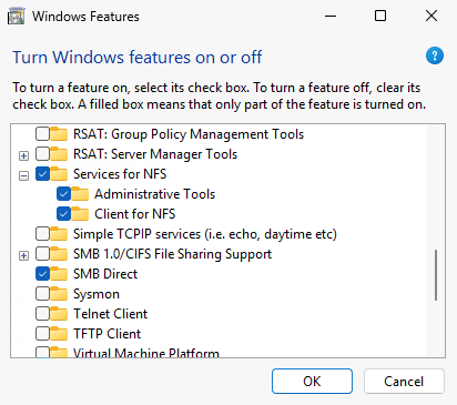
Introduction Traditional High-Performance Computing (HPC) is central to most scientific computing and engineering applications. These systems are based on well tested, repeatable, and scalable compute processes that enable the large-scale generation and validation that the semiconductor and other industries depend on. Integrating AI and agentic flows into this traditional model remains a challenge. Where many agentic systems rely on “modern” compute architecture utilizing REST based communications and object storage, traditional HPC relies on POSIX based file systems and scheduler-based orchestration. Combining these two different disciplines presents a challenge to many engineering and large-scale research enterprises. This blog describes how Microsoft Discovery app can directly interoperate with existing traditional HPC deployments utilizing Azure HPC. Microsoft Discovery is an enterprise agentic AI platform for research and development, designed to help specialized agents reason, plan, execute, and learn in a continuous loop across data, tools, and workflows. It is built on Azure and designed to integrate with capabilities such as Azure HPC and Microsoft Foundry, while leveraging industry proven tools and customer flows, making it a natural bridge between AI-native reasoning and compute-intensive engineering execution. Agentic AI in HPC The value of agentic AI in scientific and engineering workloads is not just as a chatbot or code generator; it is the ability to participate in an existing workflow: write parameter files, launch simulations, inspect logs, summarize failures, generate follow-on jobs, and preserve artifacts for traceability. To do this effectively, agents must be able also read data from POSIX-based file systems and dispatch jobs to the scheduler. To maintain IP security, they must access data while respecting the access limits of the user that dispatched them and write data under the same RBAC rules as that same user. That way organizations can be assured that agents operate strictly under the dispatching user's access rights, so they cannot reach data the user isn't authorized to see and the data they write retains the permissions that the user who dispatches the agent enjoys. Discovery app is currently only available on Windows. Linux and Mac versions will soon be available. In the meantime, enabling the Windows based Discovery app to leverage the capabilities on Azure HPC today with little to no change to the current HPC flow. Reference architecture The architecture has five primary components: a Windows VM running the Discovery app on Azure, an Azure NetApp Files volume that is mounted by both Windows and Linux clients, an Azure CycleCloud-managed HPC cluster with a Linux login node used for job submission and monitoring, and a scheduler that dispatches work to compute nodes. Discovery app on Windows: Runs on a Windows VM placed inside the same VNet, or reachable through controlled private networking, so it can access storage and the login node without exposing the HPC environment publicly. Azure NetApp Files: Provides the shared file namespace for input decks, scripts, logs, generated data, and results. Linux nodes mount the volume with native NFS. Windows can mount the same namespace through the Windows NFS client or an equivalent enterprise file-access solution. Azure CycleCloud: Provisions and manages the HPC cluster, including scheduler, login node, execute nodes, autoscaling, and cluster configuration. Login node: Acts as the controlled command endpoint. Discovery should submit jobs and query scheduler state from here, not run heavy tools directly on the login node. This protects the actual Cyclecloud scheduler and cluster manager from being overwhelmed if the dispatch volume is high. This also allows for scalability if there are many clients scheduling jobs at once. Scheduler: Incumbent schedulers that customers are already using with Azure Cyclecloud handles execution. Discovery creates scripts and submits them through the scheduler so compute runs on the correct nodes with the correct environment, licenses, and policies. This remains the same as how traditional HPC schedules jobs today. Connectivity model Running on a Windows VM in the Azure VNet aligns with many enterprises’ requirement that none of their data or IP can leave their network. Doing this avoids the need to run jobs through a user laptop or unmanaged public endpoint. This also allows the user to start an agentic workload then disconnect from the VM while the job runs and reconnect when they come back. Maintaining the same working model most engineers have with their HPC environment today. For Discovery to access Azure HPC, it needs to map the Azure NetApp Files volumes and command access to the Linux login node. File access lets agents create and read files. Command access lets agents run Linux commands, submit jobs, and monitor execution. Discovery writes execution scripts to the ANF volume, then uses SSH to dispatch the job to the schedule with the execution script. The advantage of this model is that the user can directly provide Unix-style paths to Discovery and tell it to execute tools without the user worrying about being on a Windows platform. For example, CAD teams often provide setup scripts with paths to tools that users are supposed to reference in creating their own tool execution scripts. Using this model, I just tell Discovery to use the setup script /mount/setup/tools/vendora.csh as a template and it will happily find the file and do so. I can then tell Discovery to dispatch the job to the hpc queue and it will schedule to the appropriate SLURM queue where a system is provisioned and assigned to run using the new execution script Discovery creates. This model also gets around the temporary limitation of Discovery app, unlike the enterprise Discovery service, only being available on Windows. In this model, Windows is only acting as a terminal interface so it doesn’t matter that it’s not a platform that normally works with most EDA tools. In fact, users can deploy Discovery app on either x86 or ARM Windows since all the actual tools run on the Linux-based HPC deployment in Azure anyway. Mapping Windows drive to NFS volumes Discovery agents must understand how to access files on the mapped NFS volume from the Windows VM. The same file may appear as Z:\project\run1\exec.csh on Windows and /mount/project/run1/exec.csh on Linux. The skill or instruction file used by Discovery should explicitly describe that mapping and instruct agents to use Linux paths inside batch scripts and scheduler commands. A typical instruction might say: the Windows drive Z: maps to the Linux mount point /mount. If Discovery sees /mount/designs/test.sv, it can read or write the corresponding Windows file at Z:\designs\test.sv. When generating job scripts, it should always use the Linux path, because those scripts run on the cluster. Implementation steps 1. Deploy the HPC foundation Start with the standard Azure HPC foundation: a virtual network, Azure CycleCloud, a scheduler-backed cluster, and shared storage. CycleCloud can deploy and manage Slurm clusters and supports external NFS mounts, including Azure NetApp Files. Configure the cluster so the scheduler and compute nodes mount the shared file system at a stable Linux path such as /mount, /shared, or a customer-specific project path. Make sure that systems can ssh to the login node using a public/private key pair. The login node should be accessible using a command like: % ssh -i .ssh/keyfile user@login-node 2. Place the Windows VM in the same network boundary Create a Windows VM that can reach both the Azure NetApp Files endpoint and the CycleCloud login node over private IP. The required Windows NFS client is available on Windows 11 Pro, Enterprise, and Education. It is not available on Windows 11 Home. Install the Discovery app on that VM. This VM becomes the user’s Discovery workstation for the HPC-connected workflow. Keep the VM inside the same security boundary as the HPC deployment, and use standard enterprise controls such as private networking, restricted inbound access, managed identity where appropriate, and least-privilege SSH keys. 3. Install Microsoft Discovery app Download and install Microsoft Discovery app from: https://github.com/microsoft/discovery Once installed, start Microsoft Discovery app and connect to your Github Copilot account in order to configure access to the LLM AI models. Create a new project 4. Mount the Azure NetApp Files volume into Windows Mount the same shared storage namespace into Windows. The Windows NFS client can map the NFS export to a drive letter such as Z:. The Windows NFS is sufficient for reading logs, results, and data files, and writing execution scripts, parameters, and configuration files. Heavy simulation I/O remain on Linux compute nodes running HPC tools. To configure the Windows NFS Client, you will need to have administrator privileges on your Windows VM. To mount the ANF volume with the Windows NFS client. Press Win+R Run “optional features” Select “More Windows features” Expand “Services for NFS” Enable “Administrative Tools” and “Client for NFS” Click “OK” to install the components. By default, Windows will mount the NFS volume as an anonymous user. To set the correct user, you can define the correct Linux User ID and Group ID in the registry. Note: This is an example of a functional baseline to mount a Linux volume with a user identity as an example. Production environments should employ proper identity mapping for security. Press Win+R Run “regedit” to start the Registry Editor Navigate to HKEY_LOCAL_MACHINE\SOFTWARE\Microsoft\ClientForNFS\CurrentVersion\Default In Default, right click and add two new DWORD entires: AnonymousUID and AnonymousGID Set the values to the decimal value of your Linux UID and GID. This will ensure that you connect to the ANF volume as the correct user. Select OK and then launch the Command Prompt as Administrator. To allow the NFS Client to accept the new registry entries, restart the NFS Client with the following commands: nfsadmin client stop nfsadmin client start Mount the ANF volume to a Windows drive: You should now be able to access your NFS volume by going through the Z: drive. 5. Configure SSH access to the login node Configure the SSH client on the Windows VM with a dedicated key for Discovery-driven access. The key should connect to the CycleCloud login node as the user (same as with NFS above) with permissions to submit jobs, read scheduler state, and access the shared project directory. Verify connectivity by connecting to the Cyclecloud login node using ssh from the Command Prompt. In this example, the username is ai4semi, the IP address of the login node is 10.16.16.25, and the cc_rsa is the keyfile located under the .ssh directory of the user’s home directory on Windows. Since this is the first time for this system to log into the Linux machine, you must accept the connection registration. This will not be necessary for subsequent ssh connects by Discovery using this method. 5. Teach Discovery how to use Azure HPC Now that you have the NFS and SSH connections established in Windows, you simply need to tell Discovery how to use these connections properly to run HPC workloads. In the Discovery chat window, tell Discovery to map the Z: drive on windows to the /mount volume on NFS and how to interact with the files. The Windows drive `Z:` is mapped to the cluster NFS volume `/mount`. - `/mount/<path>` on the cluster corresponds to `z:\<path>` locally. - Example: when a file is referenced as `/mount/test.txt`, look at `z:\test.txt`. Test to make sure Discovery understand by asking it to read a file on the NFS volume using POSIX nomenclature. read the contents of /mount/newfile.txt Discovery should show you the file contents Next, instruct Discovery on how to access and interact with Cyclecloud Connect to the CycleCloud login node over SSH using "ssh -i .ssh\cc_rsa ai4semi@10.16.16.25" Then tell Discovery which scheduler Cyclecloud uses and tell it to check the queue. Cyclecloud is using SLURM as the scheduler. Check the status of the hpc queue. Since the Windows VM is only used to run Discovery and the agentic AI part of the workload and the login node is not meant to run actual HPC workloads, be explicit with Discovery on how it should treat HPC job runs. NEVER run EDA/build/simulation tools on the local system or directly on the login node. ALWAYS submit work to the Slurm scheduler via sbatch. - The login node is for job submission and monitoring only — not for compute. - Wrap every tool invocation in a batch script and submit it with sbatch. 6. Validate the end-to-end workflow Validate that everything works by dispatching a simple test script to Cyclecloud Create a batch script that references the Linux path, submit it to Cyclecloud. dispatch /mount/proj/ai4semi/exec.csh to the hpc queue 7. Save the knowledge for future reference Now that Discovery understands how to access Linux-based files on NFS and how to dispatch jobs, tell it to save the information. Save this knowledge to a skill and use it for all subsequent job runs and file access for the project You see that Discovery now saved the information on how to access files and run jobs to a SKILL.md for general knowledge and updated the copilot-instructions.md to ensure that all subsequent agents and engines understand how to access Azure HPC. Note: These instructions are only scoped to a single project. When creating a new project, you can simply tell Discovery to reach over to your older project to copy the knowledge: copy over instructions on how to access NFS files and paths, and how to dispatch and execute hpc jobs from workspace1 If you want to make this a portable instruction that you can just load for each new project, tell Discovery to create a portable file. package the instructions on how to access NFS files and paths, and how to dispatch and execute hpc jobs into a a single instruction I can provide to new workspaces You can then copy the file to a central location like: C:\Users\ai4semi\project Then for each new project you can tell Discovery to use this file. read and understand the instructions in C:\Users\ai4semi\project\cyclecloud-hpc.instructions.md. Use for all agents and engines in this project and save this information as skills to use in the project Operational considerations Identity and permissions: Keep SSH access scoped to the project and avoid broad administrative privileges. For NFS, verify UID/GID mapping and file ownership behavior before production use. Performance: Use the Windows mount for orchestration artifacts, scripts, and logs. Let Linux compute nodes perform heavy I/O through native ANF mounts. Security: Keep Discovery, storage, and the login node on private networking. Avoid public exposure of scheduler or storage endpoints. Scheduler hygiene: Enforce a rule that Discovery submits jobs through the scheduler and does not run heavy tools interactively on the login node. Conclusion Connecting Microsoft Discovery app to Azure HPC allows users to seamlessly use their existing HPC environment. The most practical approach today is to place Discovery on a Windows VM inside the Azure network, map the shared Azure NetApp Files namespace into both Windows and Linux, and use SSH to submit scheduler-managed jobs through CycleCloud. Using this method, customers can quickly and easily use Discovery to integrate Agentic AI into their current HPC flows. Users can take advantage of AI agents to read and understand specification files, generate code and testbenches based on those specifications, run existing HPC tools on their Azure HPC environment. They can direct Discovery to use the scripts and resources which their CAD teams have developed. Users can create bookshelves by pointing to the documentation directories many tool vendors include in their installations, allowing Discovery to take advantage of documentation which most users don’t have time to fully digest. Over time, native Linux support can reduce the need for Windows-hosted bridging. Until then, this architecture gives teams a secure, and repeatable way to let Discovery agents create, launch, monitor, and learn from real HPC workloads on Azure.Microsoft Discovery: Where HPC meets agentic AI for the next era of EDA
Introduction High-performance computing is the engine behind the most demanding engineering breakthroughs. In electronic design automation, HPC enables massive simulation farms, verification regressions, place-and-route exploration, timing closure, power analysis, and signoff workloads that would be impractical at scale. However, as chip complexity grows, the limiting factor is no longer only compute capacity. It is the ability to reason across enormous design spaces, coordinate specialized tools, preserve engineering context, and decide what to run next. That is where Microsoft Discovery becomes especially interesting. Microsoft Discovery is an enterprise agentic AI platform for research and development, designed to help specialized agents reason, plan, execute, and learn in a continuous loop across data, tools, and workflows. It is built on Azure and designed to interoperate with capabilities such as Azure HPC and Microsoft Foundry, while leveraging industry proven tools and customer flows, making it a natural bridge between AI-native reasoning and compute-intensive engineering execution. The Inflection Point: HPC is required, but not enough Engineering teams already know how to scale compute. They run large regressions, distribute workloads across clusters, burst into cloud capacity, and optimize storage and schedulers around fast-moving design cycles. Yet the harder challenge is often deciding which simulations matter, which failures are related, which tool settings deserve another experiment, and which signals should trigger the next branch of exploration. Traditional HPC gives engineering teams scale. Agentic AI adds accelerated analysis, orchestration, memory, reasoning, and adaptation. The synthesis of the two is not about replacing engineers or replacing EDA tools. It is about turbocharging the engineers by creating an intelligent execution fabric where agents can understand goals, inspect results, choose tools, launch jobs, summarize outcomes, and recommend the next best action. Engineers remain in control of the design intent and final decisions. In this model, the most valuable resource is not compute capacity; it is engineering time. Microsoft Discovery as the agentic layer for engineering R&D Microsoft Discovery focuses on the full R&D lifecycle: knowledge reasoning, code and plan generation, simulation, analysis, and iteration. For semiconductor and EDA workflows, that maps naturally to the way design teams already operate. Timing closure, regression failure, achieving performance targets all require that engineers pour over massive amounts of information from tool run logs, interpret the results based on engineering goals and specifications, and determine how to resolve the gaps. Discovery leverages the same scientific process used in scientific research to help engineers more quickly understand the resulting data, pick out critical learnings, and help compose the next steps and mitigations. Unlike chat interfaces, agents can act and execute specific functions. Agents can be assigned roles: a verification triage agent, a log-analysis agent, a simulation-planning agent, a physical-design exploration agent, a cost-and-capacity agent, or a documentation agent that preserves evidence and rationale. Together, these agents can coordinate around a shared objective and use HPC as the execution and validation vehicle. For semiconductor programs, engineers are the most expensive and constrained part of the process. Every hour spent searching logs, reconciling reports, relaunching routine jobs, copying context between systems, or documenting repetitive findings is an hour not spent on architecture, debug strategy, design tradeoffs, or design sign-off. Discovery’s value is therefore not simply that it can automate tasks; it can help shift engineering effort away from menial coordination work and toward the decisions that improve product outcomes and silicon spins. What this looks like for EDA In a complex silicon project, design teams may run thousands of tests across multiple scenarios, configurations, simulators, and coverage targets. Today, engineers spend significant time reading logs, correlating failures, rerunning jobs, and deciding whether a failure is new, known, flaky, or blocking. Much of that work is necessary, but repetitive. With an agentic workflow, a verification agent could monitor regression output, cluster related failures, inspect logs, identify likely root causes, and propose targeted reruns rather than brute-force rerunning everything. All this helps to provide engineers more time to focus on the work that requires their unique engineering skill and judgement. In physical design, an agentic workflow could help explore constraints, placement strategies, timing violations, congestion hot spots, and power tradeoffs. HPC provides the parallel capacity to run experiments. Discovery-style agent orchestration can help determine which experiments to run, capture why they were run, compare outcomes, and refine the next set of candidates. This provides a guided design-space exploration loop. For signoff and analysis, agents could help connect results across timing, power, reliability, manufacturability, and cost. Instead of treating each report as an isolated artifact, an agentic system can reason across reports, prior runs, known design patterns, and engineering guidance helping to converge faster. Discovery leverages tried-and-true, industry-proven tools to validate the output of AI using the same methods semiconductor teams have relied on for decades. AI can propose code and plans, prioritize validation and simulation, summarize analysis and debug, or recommend next steps, but the validation path still runs through established EDA flows that engineers understand and trust. The Architecture: Agents, Tools, Data, and Compute Discovery’s flow architecture leverages a closed-loop system. Knowledge sources provide context: design specs, prior bugs, regression history, tool documentation, scripts, and engineering notes. Agents reason over that context and formulate next steps. Tool integrations connect those agents to EDA applications, schedulers, storage systems, model endpoints, and analysis pipelines. Azure HPC supplies scalable execution for simulations and compute-heavy analysis. Results flow back into the system so the next decision is better informed than the last. This demonstrates the power of joining agentic AI and HPC. Discovery provides a platform model for coordinating that loop with enterprise expectations around security, governance, transparency, and human oversight. HPC tools provide assurance that the results from AI are valid. Integrating Discovery with Azure HPC for EDA Discovery becomes even more powerful when it is connected to Azure HPC infrastructure purpose-built for compute- and memory-intensive engineering workloads. For EDA, that includes AMD-based Azure HPC virtual machines such as HX-series instances, which are optimized for silicon design and memory-intensive workloads, with large memory capacity, AMD EPYC processors with 3D V-Cache, and high-performance InfiniBand networking. These platforms give agentic workflows the execution fabric needed to run large simulations, regressions, analysis jobs, and design-space exploration at cloud scale for both EDA and other HPC workloads. Storage is equally important. EDA workloads generate and consume enormous numbers of files, and performance often depends on low-latency shared file access as much as raw CPU capacity. Azure NetApp Files provides enterprise-grade file storage for mission-critical HPC and EDA workloads in Azure, giving teams a managed, high-performance storage layer that can support simulation farms, tool installations, design libraries, scratch spaces, and shared project data. Azure NetApp Files also enables customers to use Discovery in a hybrid environment, enabling customers to keep critical data on-prem while using Discovery to optimize cloud-based flows. Many semiconductor teams keep authoritative design data, source repositories, IP libraries, and sign-off environments in on-premises infrastructure. Azure NetApp Files cache volumes can help bridge that workflow by creating a cloud-based cache of active data from an external origin volume. Frequently accessed data can be served close to Azure compute, while the authoritative dataset remains in the existing on-premises design environment. Cluster automation is another important part of enabling the hybrid flow. Azure CycleCloud can help automate the creation, scaling, and lifecycle management of HPC clusters in Azure so teams can stand up cloud capacity around specific EDA workloads rather than manually managing static infrastructure. That is important for agentic workflows because Discovery can reason about what needs to run, determine the proper resources needed, while CycleCloud-backed automation helps ensure the right compute environment is available when those jobs are ready to execute. Just as importantly, hybrid adoption does not need to force customers to replace the scheduling systems their engineering organizations already use. Many semiconductor teams have deep operational investments in incumbent schedulers which CycleCloud already works with, established queues, policies, licenses, scripts, and user workflows. A practical Discovery-plus-Azure-HPC architecture helps bring agentic AI to their existing flows: integrating cloud capacity with existing scheduler patterns, extending familiar job-submission models, and allowing teams to burst selected workloads into Azure while preserving the operational controls that have governed EDA execution for years. In that architecture, Discovery can act as the intelligent orchestration layer across the hybrid estate as well as a productivity accelerator. Agents can reason over design intent, prior results, and engineering context; submit jobs into Azure HPC environments; use AMD-powered compute for demanding EDA runs; access hot data through Azure NetApp Files; and work through cluster automation and scheduler integrations that align with customer operating models. Combined with Azure HPC, Azure NetApp Files helps eliminate storage bottlenecks that can otherwise limit EDA job throughput, allowing compute resources, EDA licenses, and engineering teams to remain productive at scale. The result is a practical synthesis: AI-guided exploration, proven EDA validation, elastic cloud compute, hybrid data access, and scheduler-aware execution that respects the way semiconductor teams already work. Why it matters for semiconductor teams Semiconductor design is a systems problem. Teams must manage more IP, more verification complexity, more software interaction, more foundry requirements, and more pressure to maintain schedules while design sizes and complexity grows. The industry has invested heavily in automation, but much of that automation remains fragmented across scripts, dashboards, job schedulers, and individual expert workflows. The simple fact is that compute is expensive, but engineering time is even more expensive. Improving engineer productivity has an outsized impact on schedule, quality, and cost. Agentic AI offers a way to automation more of the design and verification process. Automating much of the more mechanical parts of the flow. Teams can create workflows that observe, reason, and iterate while agents coordinate the results to achieve the engineering objective. Instead of relying only on tribal knowledge, teams can preserve decisions, evidence, and rationale in a repeatable workflow. Human-in-the-loop by design The goal is not autonomous chip design without engineers. The goal is amplified engineering outcomes. In the most valuable scenarios, agents handle the repetitive, high-volume, evidence-gathering work while engineers define objectives, validate assumptions, approve major decisions, and interpret tradeoffs. Discovery can help reduce the menial burden of searching, summarizing, comparing, rerunning, and documenting so engineers can spend more time on the creative and analytical work only they can do. This is especially important in EDA, where correctness, traceability, and sign-off confidence matter as much as speed. Microsoft Discovery’s emphasis on enterprise governance and transparency is therefore central to the story. In regulated or high-stakes engineering environments, teams need to know what data was used, which tools were invoked, what assumptions were made, and where human approval occurred. Just as important, they need confidence that AI-generated recommendations are validated through established engineering practices, not accepted on faith. Agentic workflows must be auditable, explainable, and grounded in the same EDA verification and signoff discipline the industry already depends on. Conclusion: Going beyond just compute and AI The next phase of EDA acceleration will not come from compute alone, and it will not come from AI alone. It will come from the synthesis of both: HPC infrastructure that can execute at scale, and agentic AI systems that can reason, coordinate, and learn across complex engineering workflows. Microsoft Discovery steps towards that future. For HPC and EDA teams, the opportunity is to move from faster batch execution to intelligent convergence: workflows that know what has been tried, understand what changed, recommend what to try next, and use scalable compute to validate ideas quickly through proven EDA tools and methodologies. In a world where design complexity keeps rising, the ability to combine elastic compute with agentic systems can help to greatly improve productivity, turn repetitive process work into guided automation, and validate AI-assisted decisions through the same trusted engineering practices the semiconductor industry has used for decades. The Microsoft Discovery team will be at Design Automation Conference, July 27-29, 2026, in Long Beach, California. The Microsoft Discovery team will be showcasing how engineers can use agentic AI to enable greater productivity for semiconductor design workloads. Drop by the Microsoft booth (651) to learn more about Microsoft Discovery for semiconductor design. Learn how technologies from AMD and NetApp come together with Azure HPC to provide the high-performance environment for running EDA tools on the cloud.AI Infrastructure Preflight at User space: Validating Multi Node, Multi GPU Slurm Clusters
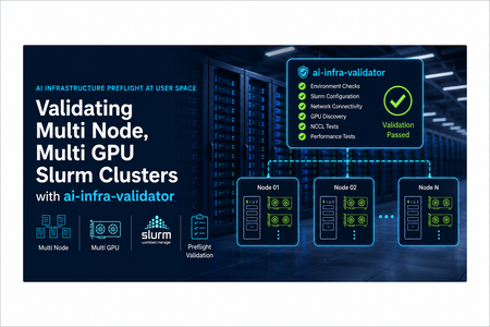
Every team that operates GPU clusters for AI has seen this pattern. The cluster boots, GPUs are visible, and scheduling works at a basic level. Then the first distributed training run stalls in NCCL initialization, fails during rank rendezvous, or silently maps ranks to the wrong devices. The issue is often not in training code. It is in infrastructure consistency across scheduler, runtime, drivers, networking, and process topology. The goal of ai-infra-validator is straightforward: Run a fast user space preflight before expensive training jobs. Validate distributed initialization for multi node, multi GPU workloads. Confirm GPU affinity and rank mapping are correct. Verify NCCL communication fabric can complete a collective ring under Slurm. This post walks through the implementation in detail, explains why each part exists, and shows how to operationalize it in real HPC AI environments. What the project validates Zero-dependency user space smoke test for AI clusters. Validates multi-node PyTorch DDP initialization, GPU affinity, and NCCL fabric connectivity under Slurm orchestration. Git Repo: ai-cluster-validator In practical terms, this checks that: Slurm launches the expected number of ranks per node. Distributed process group creation with NCCL succeeds. Each rank binds to the expected local GPU. Cross-rank all-reduce completes and converges. Node level telemetry confirms software and fabric state. This is not a performance benchmark. It is a correctness and readiness gate. Tested platform profile Component Value CycleCloud 8.8.3-3667 Slurm 25.05.5 Slurm partition hpc Scheduler VM SKU Standard_D8s_v6 Compute VM SKU Standard_ND96asr_v4 OS images microsoft-dsvm:ubuntu-hpc:2204:latest and microsoft-dsvm:ubuntu-hpc:2404:latest PyTorch 2.12.0+cu130 CUDA runtime 13.0 NCCL target 2.29.7 This profile represents a common enterprise scenario where scheduler and compute nodes have different roles, and the training fleet depends on correct multi node orchestration. Step 1: Minimal user space bootstrap The bootstrap script creates a shared Python environment at /shared/apps/pytorch_env and installs the required packages: torch torchvision torchaudio psutil This choice is intentional: No dependency on containers for first-pass validation. Single environment path visible to all compute nodes. Rapid setup and repeatability for cluster operators. Command sequence: git clone https://github.com/vinil-v/ai-cluster-validator.git cd ai-cluster-validator sudo bash bootstrap_env.sh Step 2: Slurm job defines deterministic distributed topology The Slurm script expresses a clear topology contract: nodes=2 ntasks-per-node=8 gpus-per-node=8 cpus-per-task=12 From this, world size is derived as: WORLD_SIZE = SLURM_NTASKS = 2 x 8 = 16 The script also configures network and NCCL behavior: NCCL_DEBUG=WARN NCCL_IB_DISABLE=0 NCCL_P2P_DISABLE=0 NCCL_IGNORE_CPU_AFFINITY=1 GLOO_SOCKET_IFNAME=eth0 NCCL_SOCKET_IFNAME=eth0 Important implementation detail: MASTER_ADDR is set to the first host in SLURM_JOB_NODELIST. MASTER_PORT is selected dynamically from the ephemeral range 49152-65535 and falls back to 29500 if needed. Why this matters: Reduces port collision risk when jobs run frequently. Avoids hardcoded rendezvous values that may fail in shared clusters. Launch path: srun --cpu-bind=none bash -c " source /shared/apps/pytorch_env/bin/activate; export RANK=$SLURM_PROCID; export LOCAL_RANK=$SLURM_LOCALID; python3 ddp_mesh_ping.py " The LOCAL_RANK handoff is critical for stable GPU affinity inside each node. Step 3: DDP initialization and rank to GPU affinity Inside ddp_mesh_ping.py, each process executes: Parse WORLD_SIZE, RANK, LOCAL_RANK, MASTER_ADDR, MASTER_PORT. Initialize torch.distributed with backend nccl and TCP init method. Set CUDA device using LOCAL_RANK. Core initialization path: dist.init_process_group( backend="nccl", init_method=f"tcp://{master_addr}:{master_port}", world_size=world_size, rank=rank ) torch.cuda.set_device(local_rank) This validates the minimum distributed contract required by real model training jobs. Step 4: Rich node and fabric telemetry in user space Each rank collects detailed metadata before the collective test: Node identity from Slurm and hostname. GPU model and VRAM from CUDA properties. System memory via psutil. CPU model from /proc/cpuinfo. OS and kernel versions. NVIDIA driver version from /proc/driver/nvidia/version. PyTorch, CUDA, and NCCL runtime versions. InfiniBand device state and link rate from /sys/class/infiniband. Basic GPU peer access capability via torch.cuda.can_device_access_peer. All rank payloads are gathered on rank 0 using dist.gather_object and printed as: Cluster hardware topology report. Node environment deep dive. Network interconnect and fabric status. This design gives platform teams one artifact that is both operational and diagnostic. Step 5: Functional collective validation After telemetry, each rank executes a lightweight DDP compute path: Build nn.Linear(10,10) on local GPU. Wrap with DistributedDataParallel. Perform forward, loss, backward. Run all_reduce on loss tensor. Compute global average loss. Pass condition is explicit in log output: SUCCESS: DDP Multi-Node AllReduce Ring Complete! This confirms that process group initialization and collective communication both completed successfully. What a successful run looks like Submission: sbatch ddp_smoke_test.slurm squeue Representative outcomes in the log: Total Execution Ranks: 16 Two nodes with local ranks 0 through 7 on each node GPU inventory aligned with expected A100 topology Active InfiniBand HCAs discovered per host NCCL socket interface set to eth0 Final success marker and computed convergence loss When these markers are present and coherent with expected hardware shape, the cluster is typically ready for distributed training bring-up. How to check the output file The Slurm script writes two artifacts per job: ai_infra_smoke_test_<jobid>.log ai_infra_smoke_test_<jobid>.err Use this exact workflow after submission: # 1. Submit and capture the job id sbatch ddp_smoke_test.slurm # 2. Check job state squeue -j <jobid> # 3. Read standard output log cat ai_infra_smoke_test_<jobid>.log # 4. Read standard error log cat ai_infra_smoke_test_<jobid>.err For stronger validation in automation, also check: Total Execution Ranks equals expected world size. Both nodes appear in the topology table with local ranks 0 through 7. NCCL/CUDA/PyTorch versions are present in the node environment section. Complete reference output Use the following full log as a known-good reference from a successful 2-node ND96asr_v4 run. Master Node IP/Hostname: ddpcluster-hpc-1 Dynamically Assigned Port: 53593 Total Execution Ranks: 16 =============================================================================================== HPC CLUSTER INTERACTION MONITOR =============================================================================================== --> Initializing DDP on Master Node : ddpcluster-hpc-1 --> Dynamic Coordination Port : 53593 --> Target World Cluster Size : 16 GPUs ----------------------------------------------------------------------------------------------- =============================================================================================== CLUSTER HARDWARE TOPOLOGY REPORT =============================================================================================== | Rank | Node Name | Local ID | GPU Model | VRAM | Sys Mem | CPU Cores | ----------------------------------------------------------------------------------------------- | 0 | ddpcluster-hpc-1 | 0 | NVIDIA A100-SXM4-4 | 39.5 GB | 885.8 GB | 96 Cores | | 1 | ddpcluster-hpc-1 | 1 | NVIDIA A100-SXM4-4 | 39.5 GB | 885.8 GB | 96 Cores | | 2 | ddpcluster-hpc-1 | 2 | NVIDIA A100-SXM4-4 | 39.5 GB | 885.8 GB | 96 Cores | | 3 | ddpcluster-hpc-1 | 3 | NVIDIA A100-SXM4-4 | 39.5 GB | 885.8 GB | 96 Cores | | 4 | ddpcluster-hpc-1 | 4 | NVIDIA A100-SXM4-4 | 39.5 GB | 885.8 GB | 96 Cores | | 5 | ddpcluster-hpc-1 | 5 | NVIDIA A100-SXM4-4 | 39.5 GB | 885.8 GB | 96 Cores | | 6 | ddpcluster-hpc-1 | 6 | NVIDIA A100-SXM4-4 | 39.5 GB | 885.8 GB | 96 Cores | | 7 | ddpcluster-hpc-1 | 7 | NVIDIA A100-SXM4-4 | 39.5 GB | 885.8 GB | 96 Cores | | 8 | ddpcluster-hpc-2 | 0 | NVIDIA A100-SXM4-4 | 39.5 GB | 885.8 GB | 96 Cores | | 9 | ddpcluster-hpc-2 | 1 | NVIDIA A100-SXM4-4 | 39.5 GB | 885.8 GB | 96 Cores | | 10 | ddpcluster-hpc-2 | 2 | NVIDIA A100-SXM4-4 | 39.5 GB | 885.8 GB | 96 Cores | | 11 | ddpcluster-hpc-2 | 3 | NVIDIA A100-SXM4-4 | 39.5 GB | 885.8 GB | 96 Cores | | 12 | ddpcluster-hpc-2 | 4 | NVIDIA A100-SXM4-4 | 39.5 GB | 885.8 GB | 96 Cores | | 13 | ddpcluster-hpc-2 | 5 | NVIDIA A100-SXM4-4 | 39.5 GB | 885.8 GB | 96 Cores | | 14 | ddpcluster-hpc-2 | 6 | NVIDIA A100-SXM4-4 | 39.5 GB | 885.8 GB | 96 Cores | | 15 | ddpcluster-hpc-2 | 7 | NVIDIA A100-SXM4-4 | 39.5 GB | 885.8 GB | 96 Cores | =============================================================================================== NODE ENVIRONMENT DEEP DIVE ----------------------------------------------------------------------------------------------- [ddpcluster-hpc-1] Details: --> CPU Microarchitecture : AMD EPYC 7V12 64-Core Processor --> Operating System : Ubuntu 22.04.5 LTS --> Kernel Base Version : 5.15.0-1110-azure --> Nvidia Driver Loaded : 580.126.20 --> PyTorch Environment : v2.12.0+cu130 --> CUDA Runtime Version : v13.0 --> NCCL Fabric Target : v2.29.7 --> Discovered InfiniBand HCAs: - mlx5_an0:1 (4: ACTIVE - 40 Gb/sec (4X QDR)) - mlx5_ib0:1 (4: ACTIVE - 200 Gb/sec (4X HDR)) - mlx5_ib1:1 (4: ACTIVE - 200 Gb/sec (4X HDR)) - mlx5_ib2:1 (4: ACTIVE - 200 Gb/sec (4X HDR)) - mlx5_ib3:1 (4: ACTIVE - 200 Gb/sec (4X HDR)) - mlx5_ib4:1 (4: ACTIVE - 200 Gb/sec (4X HDR)) - mlx5_ib5:1 (4: ACTIVE - 200 Gb/sec (4X HDR)) - mlx5_ib6:1 (4: ACTIVE - 200 Gb/sec (4X HDR)) - mlx5_ib7:1 (4: ACTIVE - 200 Gb/sec (4X HDR)) ----------------------------------------------------------------------------------------------- [ddpcluster-hpc-2] Details: --> CPU Microarchitecture : AMD EPYC 7V12 64-Core Processor --> Operating System : Ubuntu 22.04.5 LTS --> Kernel Base Version : 5.15.0-1110-azure --> Nvidia Driver Loaded : 580.126.20 --> PyTorch Environment : v2.12.0+cu130 --> CUDA Runtime Version : v13.0 --> NCCL Fabric Target : v2.29.7 --> Discovered InfiniBand HCAs: - mlx5_an0:1 (4: ACTIVE - 40 Gb/sec (4X QDR)) - mlx5_ib0:1 (4: ACTIVE - 200 Gb/sec (4X HDR)) - mlx5_ib1:1 (4: ACTIVE - 200 Gb/sec (4X HDR)) - mlx5_ib2:1 (4: ACTIVE - 200 Gb/sec (4X HDR)) - mlx5_ib3:1 (4: ACTIVE - 200 Gb/sec (4X HDR)) - mlx5_ib4:1 (4: ACTIVE - 200 Gb/sec (4X HDR)) - mlx5_ib5:1 (4: ACTIVE - 200 Gb/sec (4X HDR)) - mlx5_ib6:1 (4: ACTIVE - 200 Gb/sec (4X HDR)) - mlx5_ib7:1 (4: ACTIVE - 200 Gb/sec (4X HDR)) ----------------------------------------------------------------------------------------------- NETWORK INTERCONNECT & FABRIC STATUS ----------------------------------------------------------------------------------------------- --> Target Communication Interface (NCCL_SOCKET_IFNAME) : eth0 --> Active Telemetry Tracking Level (NCCL_DEBUG) : WARN --> Inter-GPU Topo Link Verification : Active (P2P/NVLink Capable) ----------------------------------------------------------------------------------------------- SUCCESS: DDP Multi-Node AllReduce Ring Complete! --> Computed System Verification Convergence Loss : 1.398719 =============================================================================================== Why this is effective for platform operations For AI infrastructure teams, this pattern is highly effective because it is: Fast: can be run after every change window. Deterministic: same topology contracts every run. Actionable: output includes enough context for first-level triage. Low friction: user space only, no heavy control plane dependencies. This supports common operating workflows: Day-0 cluster acceptance. Day-1 patch validation after driver, kernel, or image changes. Regression gate in golden image pipelines. Preflight before large multi node model training jobs. Practical guidance for extending to larger clusters Adjust Slurm directives for nodes and tasks per node. Keep one rank per GPU unless validating alternate placement policy. Set NCCL_SOCKET_IFNAME and GLOO_SOCKET_IFNAME according to your network policy. Preserve the dynamic MASTER_PORT logic to avoid static collisions. Keep the success marker string stable so automation can parse it. Closing perspective Most distributed training failures are expensive because they are discovered late. A user space preflight that validates scheduler topology, rank rendezvous, GPU affinity, and NCCL collectives provides a high value guardrail before production starts. ai-infra-validator is a practical implementation of that guardrail. It is compact, transparent, and aligned with how real Slurm based AI clusters operate. For teams running multi node multi gpu training at scale, this kind of preflight should be a standard operational gate.
Distributing model weights to your AI cluster: a faster pre-flight on AKS and Slurm
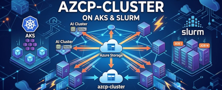
Standing up an N-node training or inference job and waiting forever for the model checkpoint to land on every node's NVMe? Here's a small Rust + MPI tool — azcp-cluster — that pays Azure egress once, broadcasts over your fabric, and finishes in seconds. Plus the AKS and Slurm patterns to wire it into a real pipeline.Simplify troubleshooting at scale - Centralized Log Management for CycleCloud Workspace for Slurm
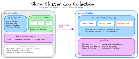
Training large AI models on hundreds or thousands of nodes introduces a critical operational challenge: when a distributed job fails, quickly identifying the root cause across scattered logs can become incredibly time-consuming. This manual process delays recovery and reduces cluster utilization. The ability to quickly parse centralized cluster logs from a single interface is critical to ensure job failure root cases are swiftly identified and mitigated to maintain high cluster utilization. Solution Architecture This is a turnkey, customizable log forwarding solution for CycleCloud Workspace for Slurm that centralizes all cluster logs into Azure Monitor Logs Analytic. The architecture uses Azure Monitor Agent (AMA) deployed on every VM and Virtual Machine Scale Set (VMSS) to stream logs defined by Data Collection Rules (DCR) to dedicated tables in a Log Analytics workspace where they can be queried from a single interface. The turnkey solution captures three categories of logs essential for troubleshooting distributed workloads, but can be extended for any other logs: Slurm logs including slurmctld, slurmd, etc., plus archived job artifacts (job submission scripts, environmental variables, stdout/stderr) collected via prolog/epilog scripts. Infrastructure logs including those from CycleCloud including the CycleCloud Healthagent which automatically tests nodes for hardware health and draining nodes that fail tests. Operation System logs from syslog and dmesg capturing kernel events, network state changes, and hardware issues. Each log source flows through its own DCR into a dedicated table following a consistent schema. The solution automatically associates scheduler-specific DCRs with the Slurm scheduler node and compute-specific DCRs with compute nodes handling dynamic node scaling transparently. The solution is purpose-built for CycleCloud Workspace for Slurm, but designed in a modular fashion to be easily extended for new data sources (i.e. new log formats) and processing (i.e. Data Collection Rules) to support log forwarding and analysis of other required logs. Key Benefits Time-series correlation: Azure Monitor's time-based indexing enables rapid identification of cascading failures. For example, trace a network carrier flap detected in syslog to corresponding slurmd communication errors to specific job failures all within seconds. Centralized visibility: Query logs from thousands of nodes through a single interface instead of SSH-ing to individual machines. Correlate Slurm controller decisions with node-level errors and system events in one query. Log persistence: Logs survive node deallocations and reimaging. Critical in cloud environments where compute nodes are ephemeral. Powerful query language: KQL (Kusto Query Language) allows parsing raw logs into structured fields, filtering across multiple sources, and building operational dashboards. Example queries detect patterns like repeated job failures, network instability, or resource exhaustion. Production-ready scalability: User-assigned managed identities automatically propagate to new VMSS instances, and DCR associations handle thousands of nodes without manual configuration. Getting Started The complete solution is available on GitHub (slurm-log-collection) with deployment scripts that: Create all required Log Analytics tables Deploys pre-configured DCRs for Slurm, CycleCloud, and OS logs Automatically associate DCRs with scheduler and compute resources After configuring environment variables and running the setup scripts, logs begin flowing to Azure Monitor and will populate within 15 minutes, but normal log ingestion latency is ~30s to 3 minutes. The repository includes sample KQL queries for common troubleshooting scenarios to accelerate time-to-resolution and to perform non-troubleshooting analysis of cluster usage.Microsoft at NVIDIA GTC 2026
Microsoft returns to NVIDIA GTC 2026 in San Jose with a strong presence across conference sessions, in‑booth theater talks, live demos, and executive‑level ancillary events. Together with NVIDIA and our partner ecosystem, Microsoft is showcasing how Azure AI infrastructure enables AI training, inference, and production at global scale. Visit us at Booth #521 to see the latest innovations in action and connect with Azure and NVIDIA experts. Exclusive GTC Experiences LEGO® Datacenter Model Explore Azure AI infrastructure at the Park Container. Candy Lounge Visit the high-traffic candy wall for co-branded treats all day long. Networking Lounge Relax and recharge with comfy seating and vital charging options. Outdoor Juice Truck Free, refreshing beverages served during outdoor park hours. Sponsored Breakout Sessions Microsoft Featured Reinventing Semiconductor Design with Microsoft Discovery S82398 · Mon, Mar 16 · 4:00 PM Prashant Varshney Microsoft · Semiconductor & AI Engineering Abstract: Semiconductor teams face exploding design complexity and shrinking verification windows. This session shows how the Microsoft Discovery AI for Science platform, combined with Synopsys Agent Engineers, introduces an agentic approach to EDA that automates routine steps and accelerates expert decision-making on Azure. Microsoft Featured Operationalizing Agentic AI at Hyperscale S82399 · Tue, Mar 17 · 1:00 PM Nitin Nagarkatte Microsoft · Azure AI Infrastructure Anand Raman Microsoft · Azure AI Vipul Modi Microsoft · AI Systems Abstract: As enterprises move to agentic systems, the challenge shifts to operating intelligent agents reliably at scale. This session demonstrates how Microsoft builds AI Factories on Azure using NVIDIA technology and explores Microsoft Foundry as the control plane for deploying and operating coordinated AI agents. Live from GTC: AI Podcast Dayan Rodriguez Corporate Vice President Global Manufacturing and Mobility Alistair Spiers General Manager Azure Infrastructure Live Special Feature A conversation with Microsoft Azure Listen & Subscribe: aka.ms/GTC2026Podcast Scan to Listen Earned Conference Sessions Don't miss these high-impact sessions where Microsoft and NVIDIA leaders discuss the future of AI factories and infrastructure. Mon · Mar 16 5:00 PM Drive Optimal Tokens per Watt on AI Infrastructure Using Benchmarking Recipes Speakers: Paul Edwards, Emily Potyraj Microsoft, NVIDIA Tue · Mar 17 9:00 AM Autonomous AI Factories: Technical Preview of Agent-Native Production Speakers: JP Vasseur, César Martinez Spessot NVIDIA, Microsoft Research Tue · Mar 17 4:00 PM The Road to Intelligent Mobility: Vehicle GenAI Speakers: Raj Paul, Thomas Evans, Bryan Goodman Microsoft, NVIDIA, Bosch Wed · Mar 18 9:00 AM Supercharging AI with Multi-Gigawatt AI Factories Speakers: Gilad Shainer, Peter Salanki, Evan Burness NVIDIA, CoreWeave, Meta, Microsoft Daily Booth Theater Schedule Visit the Microsoft Theater for lightning talks from engineering leaders and partners. Monday, March 16 2:00 PM BTH208 · NVIDIA Accelerate AI Innovation on Azure with NVIDIA Run:ai — Rob Magno 2:30 PM BTH202 · General Robotics Models to Machines: Deploying Agentic AI in Real-World Robotics — Dinesh Narayanan 3:00 PM BTH200 · Fractal Analytics From Generalist to Enterprise-Ready: Fractal Builds Domain AI — C. Chaudhuri 3:30 PM BTH109 · Microsoft Agentic cloud ops - Smarter Operations with Azure Copilot — Jyoti Sharma 4:00 PM BTH103 · Microsoft Build a Deep Research Agent for Enterprise Data — D. Casati, A. Slutsky, H. Alkemade 4:30 PM BTH205 · NetApp Azure NetApp Files: Powering Your Data for AI Capabilities — Andy Chan 5:00 PM BTH207 · NVIDIA The Agentic Commerce Stack: Open Models on Azure — Antonio Martinez 5:30 PM BTH217 · OPAQUE Confidential AI on Azure Unlocks Sovereign AI at Scale — Aaron Fulkerson 6:00 PM BTH218 · Simplismart Making BYOC work at scale with modular inference — Amritanshu Jain 6:30 PM Expo Reception Tuesday, March 17 1:30 PM BTH100 · Microsoft From Open Weights to Enterprise Scale: Open-Source Models — Sharmila Chockalingam 2:00 PM BTH212 · Personal AI Unlocking the power of memory in Teams with Personal AI — Sam Harkness 2:30 PM BTH111 · Microsoft / NVIDIA Scalable LLM Inference on AKS Using NVIDIA Dynamo — Mohamad Al jazaery, Anton Slutsky 3:00 PM BTH204 · Mistral AI Innovate with Mistral AI on Microsoft Foundry — Ian Mathew 3:30 PM BTH104 · Microsoft GPU-Accelerated CFD at Scale: Star-CCM+ on Azure — Jason Scheffelmaer 4:00 PM BTH206 · NeuBird AI Agentic AI for Incident Response on Microsoft Azure — Grant Griffiths 4:30 PM BTH101 · GitHub Agentic DevOps: Evolving software with GitHub Copilot — Glenn Wester 5:00 PM BTH209 · Rescale Real-World AI Physics: GM & NVIDIA on Rescale — Dinal Perera 5:30 PM BTH107 · Microsoft Intro to LoRA Fine-Tuning on Azure — Christin Pohl 6:30 PM Raffle Wednesday, March 18 1:00 PM BTH219 · VAST Data Scaling AI Infrastructure on Azure with VAST Data — Jason Vallery 1:30 PM BTH110 · Microsoft Physical AI and Robotics: The Next Frontier — F. Miller, C. Souche, D. Narayanan 2:00 PM BTH105 · Microsoft Sovereign AI options with Azure Local — Kim Lam 2:30 PM BTH108 · Microsoft Automating HPC Workflows with Copilot Agents — Param Shah 3:00 PM BTH102 · Microsoft Trustworthy Multi-Agent Workflows with Microsoft Foundry — Brian Benz 4:00 PM BTH106 · Microsoft Scaling Enterprise AI on ARO with NVIDIA H100 & H200 — Lachie Evenson 4:30 PM BTH211 · WEKA Hybrid AI Data Orchestration with WEKA NeuralMesh™ — Desiree Campbell 5:00 PM BTH202 · Hammerspace NVIDIA AI Enterprise Software with NIM — Mike Bloom 5:30 PM BTH203 · Kinaxis Reimagining Global Supply Planning with Azure — Dane Henshall 6:00 PM BTH214 · AT&T Connected AI on Azure for Manufacturing — Brad Pritchett 6:30 PM Raffle Thursday, March 19 11:00 AM BTH210 · Wandelbots Physical AI: Powering Software-Defined Automation in Robotics — Marwin Kunz, Martin George 11:30 AM Raffle Explore Our Demo Pods Visit the Microsoft booth to see our technology in action with live demonstrations across four dedicated pod areas. POD 1 Azure AI Infrastructure End‑to‑end AI infrastructure for training and inference at scale, featuring the latest NVIDIA GPU integrations on Azure. POD 2 Microsoft Foundry Our comprehensive platform for building, deploying, and operating agentic AI systems with enterprise reliability. POD 3 Building AI Together Showcasing joint Microsoft and NVIDIA solutions across diverse industries, from manufacturing to retail. POD 4 Startups Powering AI Discover how innovative startups are running next‑generation AI workloads on the Azure platform. Ancillary Events & Networking Join Microsoft leadership and our partner ecosystem at these curated networking experiences. Click the location to view on Bing Maps. Sun · Mar 15 6:00 PM Microsoft for Startups Executive Leadership Dinner 📍 Morton’s Steakhouse, San Jose Exclusive gathering for startup leaders and Microsoft executives. Mon · Mar 16 1:30 PM Microsoft × NVIDIA Open Meet 📍 Signia by Hilton · International Suite Strategic alignment session for Microsoft and NVIDIA executives. Mon · Mar 16 7:30 PM Microsoft + NVIDIA Executive Dinner 📍 Il Fornaio, San Jose Executive dinner for key customers and leadership teams. Tue · Mar 17 11:00 AM to 1:00 PM Microsoft AI Luncheon: Research, Robotics, & Real‑World AI 📍 Signia by Hilton · International Suite Invite-only: A curated executive lunch exploring the journey from AI research to physical enterprise deployments in robotics and manufacturing. Tue · Mar 17 7:30 PM Networking in AI & Tech 📍 San Pedro Square Market Community networking mixer for Microsoft teams, partners, and customers. Wed · Mar 18 10:00 AM to 1:00 PM AI Innovator’s Circle Brunch: Powering Intelligent Systems Across the Ecosystem 📍 Il Fornaio, San Jose Hosted by Microsoft & NVIDIA at GTC. Join us for an exclusive brunch and discussion on the intelligent ecosystem.
Centralized cluster performance metrics with ReFrame HPC and Azure Log Analytics
Imagine having several clusters across different environments (dev, test and prod) or planning a migration between PBS and Slurm or porting codes to a different system. They can all seem like daunting tasks. This is where the combination of ReFrame HPC, a powerful and feature rich testing framework, and Azure Log Analytics can help improve confidence and assurance in the performance and accuracy of a system. Here we will look at how to configure ReFrame HPC specifically for Azure: Deploying the required Azure resources, running a test and capturing the results in Log Analytics for analysis. Deploying the required Azure Resources Firstly, deploy the required resources in Azure by using this bicep from GitHub. The deployment includes the creation and configuration of everything required for ReFrame HPC. These resources include a data collection endpoint, a data collection rule and a log analytics workspace. Running ior via ReFrame HPC For the purpose of demonstrating a running test and capturing the results in Azure from start to finish, here is a simple ior test which will run both a read and a write operation against the shared storage. import reframe as rfm import reframe.utility.sanity as sn @rfm.simple_test class SimplePerfTest(rfm.RunOnlyRegressionTest): valid_systems = ["*"] valid_prog_environs = ["+ior"] executable = 'ior' executable_opts = [ '-a POSIX -w -r -C -e -g -F -b 2M -t 2M -s 25600 -o /data/demo/test.bin -D 300' ] reference = { 'tst:hbv4': { 'write_bandwidth_mib': (500, -0.05, 0.1, 'MiB/s'), 'read_bandwidth_mib': (350, -0.05, 0.5, 'MiB/s'), } } @sanity_function def validate_run(self): return sn.assert_found(r'Summary of all tests:', self.stdout) @performance_function('MiB/s') def write_bandwidth_mib(self): return sn.extractsingle(r'^write\s+([0-9]+\.?[0-9]*)', self.stdout, 1, float) @performance_function('MiB/s') def read_bandwidth_mib(self): return sn.extractsingle(r'^read\s+([0-9]+\.?[0-9]*)', self.stdout, 1, float) Test explanation Set the binary to be executed to ior, along with its arguments. executable = 'ior' executable_opts = [ '-a POSIX -w -r -C -e -g -F -b 2M -t 2M -s 25600 -o /data/demo/test.bin -D 300' ] Specify which systems the test should run on. In this case, any system/cluster which is known to have ior available will be selected. Look at the ReFrame HPC documentation to get a better understanding of the options available for use. valid_systems = ["*"] valid_prog_environs = ["+ior"] Verify the stdout of the job by searching for a specific value to assert that it ran successfully. @sanity_function def validate_run(self): return sn.assert_found(r'Summary of all tests:', self.stdout) If the sanity function passed it will then extract the performance metrics from the stdout of the job. The naming of the methods is important, as they will be stored in the results later. @performance_function('MiB/s') def write_bandwidth_mib(self): return sn.extractsingle(r'^write\s+([0-9]+\.?[0-9]*)', self.stdout, 1, float) @performance_function('MiB/s') def read_bandwidth_mib(self): return sn.extractsingle(r'^read\s+([0-9]+\.?[0-9]*)', self.stdout, 1, float) Performance references are used to determine if the current cluster has met the requirement or not. It also allows margins to be specified in either direction. reference = { 'tst:hbv4': { 'write_bandwidth_mib': (500, -0.05, 0.1, 'MiB/s'), 'read_bandwidth_mib': (350, -0.05, 0.5, 'MiB/s'), } } ReFrame HPC Configuration The ReFrame HPC configuration is key to determine how and where the test will run. It is also where the logic allowing Reframe HPC to use Azure for centralized logging will be defined. The full configuration file is vast and is covered in detail within the ReFrame HPC documentation. For the purpose of this test an example can be found on GitHub. Below is a breakdown of the key parts that allow Reframe HPC to push its results into Azure Log Analytics. Logging Handler The most important part of this configuration is the logging section, without it ReFrame HPC will not attempt to log the results. A handler_perflog of type httpjson is added to enable the logs to be sent to a HTTP endpoint with specific values which our covered below. 'logging': [ { 'perflog_multiline': True, 'handlers_perflog': [ { 'type': 'httpjson', 'url': 'REDACTED', 'level': 'info', 'debug': False, 'extra_headers': {'Authorization': f'Bearer {_get_token()}'}, 'extras': { 'TimeGenerated': f'{datetime.now(timezone.utc).isoformat()}', 'facility': 'reframe', 'reframe_azure_data_version': '1.0', }, 'ignore_keys': ['check_perfvalues'], 'json_formatter': _format_record } ] } Multiline Perflog To ensure this works with Azure, enable perflog_multiline. This will ensure a single record per metric is sent to Log Analytics. This is the cleanest way to output the results. Having this set to False will move the metric names into column names, which means that the schema will be different for each test and will become hard to maintain. Extra Headers A bearer token is required to authenticate the request. ReFrame HPC allows the adding of headers via the extra_headers property and a simple Python function, which obtains a scoped token that can be appended to the additional header. def _get_token(scope='https://monitor.azure.com/.default') -> str: credential = DefaultAzureCredential() token = credential.get_token(scope) return token.token Url Structure The url can be found in the output of the bicep which was run previously. It can also be obtained via the portal. Here is the structure of the url for reference. '${dce.properties.logsIngestion.endpoint}/dataCollectionRules/${dcr.properties.immutableId}/streams/Custom-${table.name}?api-version=2023-01-01' json Formatter A small work around is needed as the Data Collection Rule expects an array of items and ReFrame HPC outputs a single record. To resolve this another Python function can be used which simply wraps the record up in an array. In this example it also tidys up and removes some items that are not required and would cause issues with the json serialization. def _format_record(record, extras, ignore_keys): data = {} for attr, val in record.__dict__.items(): if attr in ignore_keys or attr.startswith('_'): continue data[attr] = val data.update(extras) return json.dumps([data]) Running the Test Now that the infrastructure has been deployed, the test has been defined and is correctly configured, we can run the test. Start by logging in. Here I am using the managed identity of the node, but User auth and User Assigned Managed Identities are also supported. $ az login --identity ReFrame HPC can be installed via Spack or Python and, while I am using Spack for packages on the cluster, I find the simplest approach is to activate a Python environment and install ReFrame HPC along with test specfic Python dependencies. $ python3 -m venv .venv $ . .venv/bin/activate $ python -m pip install -U pip $ pip install -r requirements.txt Now using the ReFrame HPC cli, the test can be run using the configuration file and the test file. $ reframe -C config.py -c simple_perf.py --performance-report -r ReFrame HPC will now run the test against the system/cluster defined in the configuration. For this example it is a Slurm cluster on a partition of HBv4 nodes and running squeue clarifys that. $ squeue JOBID PARTITION NAME USER ST TIME NODES NODELIST(REASON) 955 hbv4 rfm_Simp jim.pain R 0:28 1 tst4-hbv4-97 Results And there we have it, results are now appearing in Azure! From here we can use kql to query and filter the results. This is just a subset of the values available but the dataset is vast and includes a huge range of values that are extremely helpful. Summary By standardizing on the combination of ReFrame HPC and Azure Log Analytics for testing and reporting of performance data across our clusters, whether Slurm based, Azure CycleCloud or existing on-prem clusters, you can gain unprecendented visibility and confidence in the systems you manage and the codes you deploy that were previously hard to obtain. Enabling the potential for: 🔎Fast cross-cluster comparisions 📈Trend analysis over long running periods 📊Standardized metrics regardless of scheduler or system ☁️Unified monitoring and reporting across clusters ReFrame HPC is suitable for a wide range of testing, so if testing is something you have been looking to implement, take a look at ReFrame HPCScaling physics-based digital twins: Neural Concept on Azure delivers a New Record in Industrial AI
Automotive Design and the DrivAerNet++ Benchmark In automotive design, external aerodynamics have a direct impact on performance, energy efficiency, and development cost. Even small reductions in drag can translate into significant fuel savings or extended EV range. As development timelines accelerate, engineering teams increasingly rely on data-driven methods to augment or replace traditional CFD workflows. MIT’s DrivAerNet++ dataset is the largest open multimodal dataset for automotive aerodynamics, offering a large-scale benchmark for evaluating learning-based approaches that capture the physical signals required by engineers. It includes 8,000 vehicle geometries across 3 variants (fastback, notchback and estate-back) and aggregates 39 TB of high-fidelity CFD outputs such as surface pressure, wall shear stress, volumetric flow fields, and drag coefficients. Benchmark Highlights Neural Concept trained its geometry-native Geometric Regressor, designed to handle any type of engineering data. The benchmark was executed on Azure HPC infrastructure to evaluate the capabilities of the geometry-native platform under transparent, scalable, and fully reproducible conditions. Surface pressure: Lowest prediction error recorded on the benchmark, revealing where high- and low-pressure zones form. Wall shear stress: Outperforming all competing methods to detect flow attachment and separation for drag and stability control. Volumetric velocity field: More than 50% lower error than previous best, capturing full flow structure for wake stability analysis. Drag coefficient Cd: R² of 0.978 on the test set, accurate enough for early design screening without full CFD runs. Dataset Scale and Ingestion: 39 TB of data was ingested into Neural Concept’s platform through a parallel conversion task with 128 workers and 5 GB RAM each that finished in about 1 hour and produced a compact 3 TB dataset in the platform’s native format. Data Pre Processing: Pre-processing the dataset required both large-scale parallelization and the application of our domain-specific best practices for handling external aerodynamics workflows. Model Training and Deployment: Training completed in 24 hours on 4 A100 GPUs, with the best model obtained after 16 hours. The final model is compact and real-time predictions can be served on a single 16 GB GPU for industrial use. Neural Concept outperformed all other competing methods, achieving state-of-the-art performance prediction on all metrics and physical quantities within a week: “Neural Concept’s breakthrough demonstrates the power of combining advanced AI with the scalability of Microsoft Azure,” said Jack Kabat, Partner, Azure HPC and AI Infrastructure Products, Microsoft. “By running training and deployment on Azure’s high-performance infrastructure — specifically the NC A100 Virtual Machine— Neural Concept was able to transform 39 terabytes of data into a production-ready workflow in just one week. This shows how Azure accelerates innovation and helps automotive manufacturers bring better products to market faster.” For additional benchmark metrics and comparisons, please refer to the Detailed Quantitative Results section at the end of the article. From State-Of-The-Art Benchmark Accuracy to Proven Industrial Impact Model accuracy alone is necessary, but not sufficient for industrial impact. Transformative gains at scale and over time are only revealed once high-performing models are deployed into maintainable and repeatable workflows across organizations. Customers using Neural Concept’s platform have achieved: 30% shorter design cycles $20M in savings on a 100,000-unit vehicle program These outcomes fundamentally result from a transformed, systematic approach to design, unlocking better and faster data-driven decisions. The Design Lab interface, described in the next section, is at the core of this transformation. Within Neural Concept’s ecosystem, validated geometry and physics models can be deployed directly into the Design Lab - a collaborative environment where aerodynamicists and designers evaluate concepts in real time. AI copilots provide instant performance feedback, geometry-aware improvement suggestions, and live KPI updates, effectively reconnecting aerodynamic analysis with the pace of modern vehicle design. CES 2026: See how OEMs are transforming product development with Engineering Intelligence Neural Concept and Microsoft will showcase how AI-native aerodynamic workflows can reshape vehicle development — from real-time design exploration to enterprise-scale deployment. Visit the Microsoft booth to see DrivAerNet++ running on Azure HPC and meet the teams shaping the future of automotive engineering. Visit Microsoft Booth to find out more Neural Concept’s executive team will also be at CES to share flagship results achieved by leading OEMs and Tier-1 suppliers already using the platform in production. Learn more on: https://www.neuralconcept.com/ces-2026 Credits Microsoft: Hugo Meiland (Principal Program Manager), Guy Bursell (Director Business Strategy, Manufacturing), Fernando Aznar Cornejo (Product Marketing Manager) and Dr. Lukasz Miroslaw (Sr. Industry Advisor) Neural Concept: Theophile Allard (CTO), Benoit Guillard (Senior ML Research Scientist), Alexander Gorgin (Product Marketing Engineer), Konstantinos Samaras-Tsakiris (Software Engineer) Detailed Quantitative Results In the sections that follow, we share the results obtained by applying Neural Concept’s aerodynamics predictive model training template to Drivaernet++. We evaluated our model’s prediction errors using the official train/test split and the standard evaluation strategy. For comparison, metrics from other methods were taken from the public leaderboard. We reported both Mean Squared Error (MSE) and Mean Absolute Error (MAE) to quantify prediction accuracy. Lower values for either metric indicate closer agreement with the ground truth simulations, meaning better predictions. 1. Surface Field Predictions: Pressure and Wall Shear Stress We began by evaluating predictions for the two physical quantities defined on the vehicle surface. Surface Pressure The Geometric Regressor achieved substantially better performance than all existing methods in predicting surface pressure distribution. Rank Deep Learning Model MSE (*10-2, lower = better) MAE (*10-1, lower = better) #1 Neural Concept 3.98 1.08 #2 GAOT (May 2025) 4.94 1.10 #3 FIGConvNet (February 2025) 4.99 1.22 #4 TripNet (March 2025) 5.14 1.25 #5 RegDGCNN (June 2024) 8.29 1.61 Table 1: Neural Concept’s Geometric Regressor predicts surface pressure more accurately than previously published state-of-the-art methods. The dates indicate when the competing model architectures were published. Figure 1: Side-by-side comparison of the ground truth pressure field (left), Neural Concept model’s prediction (middle), and the corresponding error for a representative test sample (right). Wall Shear Stress Similarly, the model delivered top-tier results, outperforming all competing methods. Rank Deep Learning Model MSE (*10 -2 , lower = better) MAE (*10 -1 , lower = better) #1 Neural Concept 7.80 1.44 #2 GAOT (May 2025) 8.74 1.57 #3 TripNet (March 2025) 9.52 2.15 #4 FIGConvNet (Feb. 2025) 9.86 2.22 #5 RegDGCNN (June 2024) 13.82 3.64 Table 2: Neural Concept’s Geometric Regressor predicts wall shear stress more accurately than previously published state-of-the-art methods. Figure 2: Side-by-side comparison of the ground truth magnitude of the wall shear stress, Neural Concept model’s prediction, and the corresponding error for a representative test sample. Across both surface fields (pressure and wall shear stress), the Geometric Regressor achieved the lowest MSE and MAE by a clear margin. The baseline methods represent several high-quality and recent academic work (the earliest being from June 2024), yet our architecture established a new state-of-the-art in predictive performance. 2. Volumetric Predictions: Velocity Beyond surface quantities, DrivAerNet++ provides 3D velocity fields in the flow volume surrounding the vehicle, which we also predicted using the Geometric Regressor. Rank Deep Learning Model MSE (lower = better) MAE (*10 -1 , lower = better) #1 Neural Concept 3.11 9.22 #2 TripNet (March 2025) 6.71 15.2 Table 3: Neural Concept’s Geometric Regressor predicts velocity more accurately than the previously published state-of-the-art method. The illustration below shows the velocity magnitude for two test samples. Note that only a single 2D slice of the 3D volumetric domain is shown here, focusing on the wake region behind the car. In practice, the network predicts velocity at any location within the full 3D domain, not just on this slice. Figure 3: Velocity magnitude for two test samples, arranged in two columns (left and right). For each sample, the top row displays the simulated velocity field, the middle row shows the prediction from the network, and the bottom row presents the error between the two. 3. Scalar Predictions: Drag Coefficient The drag coefficient (Cd) is the most critical parameter in automotive aerodynamics, as reducing it directly translates to lower fuel consumption in combustion vehicles and increased range in electric vehicles. Using the same underlying architecture, our model achieved state-of-the-art performance in Cd prediction. In addition to MSE and MAE, we reported the Maximum Absolute Error (Max AE) to reflect worst-case accuracy. We also included the Coefficient of Determination (R² score), which measures the proportion of variance explained by the model. An R² value of 1 indicates a perfect fit to the target data. Rank Deep Learning Model MSE (*1e-5) MAE (*1e-3) Max AE (*1e-2) R² #1 Neural Concept 0.8 2.22 1.13 0.978 #2 TripNet 9.1 7.19 7.70 0.957 #3 PointNet 14.9 9.60 12.45 0.643 #4 RegDGCNN 14.2 9.31 12.79 0.641 #5 GCNN 17.1 10.43 15.03 0.596 On the official split, the model shows tight agreement with CFD (R² of 0.978) across the test set, which is sufficient for early design screening where engineers need to rank variants confidently and spot meaningful gains without running full simulations for every change. 4. Compute Efficiency and Azure HPC&AI Collaboration Executing the full DrivAerNet++ benchmark at industrial scale required Neural Concept’s full software and infrastructure stack combined with seamless cloud integration on Microsoft Azure to dynamically scale computing resources on demand. The entire pipeline runs natively on Microsoft Azure and can scale within minutes, allowing us to process new industrial datasets that contain thousands of geometries without complex capacity planning. Dataset Scale and Ingestion DrivAerNet++ dataset contains 8000 car designs along with their corresponding CFD simulations. The raw dataset occupies approximately 39TB of storage. Generating the simulations required a total of about 3 million CPU hours by MIT’s DeCoDE Lab. Ingestion into Neural Concept’s platform is the first step of the pipeline. To convert the raw data into the platform’s native format, we use a Conversion task that transforms raw files into the platform’s optimized native format. This task was parallelized with 128 workers; each allocated 5 GB of RAM. As a result, the entire conversion process was completed in approximately one hour only. After converting the relevant data (car geometry, wall shear stress, pressure, and velocity), the full dataset occupies approximately 3 TB in Neural Concept’s native format. Data Pre-Processing Pre-processing the dataset required both large-scale parallelization and the application of our domain-specific best practices. During this phase, workloads were distributed across multiple compute nodes with peak memory usage reaching approximately 1.5 TB of RAM. The pre-processing pipeline consists of two main stages. In the first stage, we repaired the car meshes and pre-computed geometric features needed for training. The second stage involved filtering the volumetric domain and re-sampling points to follow a spatial distribution that is more efficient for training our deep learning model. We scaled the compute resources so that each of the two stages in the pipeline completes in 1 to 3 hours when processing the full dataset. The first stage is the most computationally intensive. To handle it efficiently, we parallelized the task across 256 independent workers, each allocated 6 GB of RAM. Model Training and Deployment While we use state-of-the-art hardware for training, our performance gains come primarily from model design. Once trained, the model remains lightweight and cost-effective to run. Training was performed on Azure Standard_NC96ads_A100_v4 node, which provided access to four A100 GPUs, each with 80 GB of memory. The model was trained for approximately 24 hours. Neural Concept’s Geometric Regressor achieved the best reported performance on the official benchmark for surface pressure, wall shear stress, volumetric velocity and drag prediction.