azure sql database

561 Topics

Stop defragmenting and start living: auto index compaction is now generally available
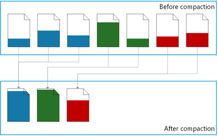
Executive summary Automatic index compaction is a built-in MSSQL database engine feature that compacts indexes in background and with minimal overhead. Now you can: Stop using scheduled index maintenance jobs. Reduce storage space consumption and save costs. Improve performance by reducing CPU, memory, and disk I/O consumption. Automatic index compaction is now generally available in Azure SQL Database, Azure SQL Managed Instance with the always-up-to-date update policy, and SQL database in Fabric. Index maintenance without maintenance jobs Enable automatic index compaction for a database with a single T-SQL command: ALTER DATABASE [database-name] SET AUTOMATIC_INDEX_COMPACTION = ON; Once enabled, you no longer need to set up, maintain, and monitor resource intensive index maintenance jobs, a time-consuming operational task for many DBA teams today. As the data in the database changes, a background process consolidates rows from partially filled data pages into a smaller number of filled up pages, and then removes the empty pages. Index bloat is eliminated – the same amount of data now uses a minimal amount of storage space. Resource consumption is reduced because the database engine needs fewer disk IOs and less CPU and memory to process the same amount of data. By design, the background compaction process acts on the recently modified pages only. This means that its own resource consumption is much lower compared to the traditional index maintenance operations (index rebuild and reorganize), which process all pages in an index or its partition. For a detailed description of how the feature works, a comparison between automatic index compaction and the traditional index maintenance operations, and the ways to monitor the compaction process, see automatic index compaction in documentation. Let the numbers speak As auto index compaction becomes generally available, it is already enabled in more than 6 million databases worldwide, most of them from Microsoft internal customers who helped validate the feature during preview. Hundreds of external customers also enabled auto compaction during preview and have been enjoying the benefits, with zero issues reported. Looking at our worldwide telemetry data for a 28-day window, automatic index compaction freed up approximately 14.3 petabytes of space in data files by consolidating 547.5 trillion rows on fewer pages, saving resources and improving query performance. Looking at the space freed up per database, the benefits range from a few megabytes per day for databases with already dense pages, to more than 500 gigabytes per day for databases that have gone through one-time extensive data modifications. Compaction in action To see the effects of automatic index compaction, we wrote a stored procedure that simulates a write-intensive OLTP workload. Each execution of the procedure inserts, updates, deletes, or selects a random number of rows, from 1 to 100, in a 50,000-row table with a clustered index. We executed this stored procedure using a popular SQLQueryStress tool, with 30 threads and 400 iterations on each thread. We measured the page density, the number pages in the leaf level of the table’s clustered index, and the number of logical reads (pages) used by a test query reading 1,000 rows, at three points in time: After initially inserting the data and before running the workload. Once the workload stopped running. Several minutes later, once the background process completed index compaction. Here are the results: Before workload After workload After compaction Logical reads 25 🟢 1,610 🔴⬆️ 35 🟢⬇️ Page density 99.51% 🟢 52.71% 🔴⬇️ 96.11% 🟢⬆️ Pages 962 🟢 4,394 🔴⬆️ 1,065 🟢⬇️ Before the workload starts, page density is high because nearly all pages are full. The number of logical reads required by the test query is minimal, and so is its resource consumption. The workload leaves a lot of empty space on pages and increases the number of pages because of row updates and deletions, and because of page splits. As a result, immediately after workload completion, the number of logical reads required for the same test query increases more than 60 times, which translates into a higher CPU and memory usage. But then within a few minutes, automatic index compaction removes the empty space from the index, increasing page density back to nearly 100%, reducing logical reads by about 98% and getting the index very close to its initial compact state. Less logical reads means that the query is faster and uses less CPU. All of this without any user action. With continuous workloads, index compaction is continuous as well, maintaining higher average page density and reducing resource usage by the workload over time. The T-SQL code we used in this demo is available in the Appendix. Conclusion Automatic index compaction delegates a routine database maintenance operation to the database engine itself, letting administrators and engineers focus on more important work without worrying about index maintenance. Making this feature generally available doesn’t mean that we stop working on it. Your feedback during preview helped us find new opportunities to fine-tune the compaction process. We thank you for that feedback and look forward to announcing new improvements in auto index compaction in the future. Appendix Here is the T-SQL code we used to demonstrate automatic index compaction. The type of executed statements and the number of affected rows is randomized to better represent an OLTP workload. While the results demonstrate the effectiveness of automatic index compaction, exact measurements may vary from one execution to the next. /* Enable automatic index compaction */ ALTER DATABASE CURRENT SET AUTOMATIC_INDEX_COMPACTION = ON; /* Reset to the initial state */ DROP TABLE IF EXISTS dbo.t; DROP SEQUENCE IF EXISTS dbo.s_id; DROP PROCEDURE IF EXISTS dbo.churn; /* Create a sequence to generate clustered index keys */ CREATE SEQUENCE dbo.s_id AS int START WITH 1 INCREMENT BY 1; /* Create a test table */ CREATE TABLE dbo.t ( id int NOT NULL CONSTRAINT df_t_id DEFAULT (NEXT VALUE FOR dbo.s_id), dt datetime2 NOT NULL CONSTRAINT df_t_dt DEFAULT (SYSDATETIME()), u uniqueidentifier NOT NULL CONSTRAINT df_t_uid DEFAULT (NEWID()), s nvarchar(100) NOT NULL CONSTRAINT df_t_s DEFAULT (REPLICATE('c', 1 + 100 * RAND())), CONSTRAINT pk_t PRIMARY KEY (id) ); /* Insert 50,000 rows */ INSERT INTO dbo.t (s) SELECT REPLICATE('c', 50) AS s FROM GENERATE_SERIES(1, 50000); GO /* Create a stored procedure that simulates a write-intensive OLTP workload. */ CREATE OR ALTER PROCEDURE dbo.churn AS SET NOCOUNT, XACT_ABORT ON; DECLARE @r float = RAND(CAST(CAST(NEWID() AS varbinary(4)) AS int)); /* Get the type of statement to execute */ DECLARE @StatementType char(6) = CASE WHEN @r <= 0.15 THEN 'insert' WHEN @r <= 0.30 THEN 'delete' WHEN @r <= 0.65 THEN 'update' WHEN @r <= 1 THEN 'select' ELSE NULL END; /* Get the maximum key value for the clustered index */ DECLARE @MaxKey int = ( SELECT CAST(current_value AS int) FROM sys.sequences WHERE name = 's_id' AND SCHEMA_NAME(schema_id) = 'dbo' ); /* Get a random key value within the key range */ DECLARE @StartKey int = 1 + RAND() * @MaxKey; /* Get a random number of rows, between 1 and 100, to modify or read */ DECLARE @RowCount int = 1 + RAND() * 99; /* Execute a statement */ IF @StatementType = 'insert' INSERT INTO dbo.t (id) SELECT NEXT VALUE FOR dbo.s_id FROM GENERATE_SERIES(1, @RowCount); IF @StatementType = 'delete' DELETE TOP (@RowCount) dbo.t WHERE id >= @StartKey; IF @StatementType = 'update' UPDATE TOP (@RowCount) dbo.t SET dt = DEFAULT, u = DEFAULT, s = DEFAULT WHERE id >= @StartKey; IF @StatementType = 'select' SELECT TOP (@RowCount) id, dt, u, s FROM dbo.t WHERE id >= @StartKey; GO /* The remainder of this script is executed three times: 1. Before running the workload using SQLQueryStress. 2. Immediately after the workload stops running. 3. Once automatic index compaction completes several minutes later. */ /* Monitor page density and the number of pages and records in the leaf level of the clustered index. */ SELECT avg_page_space_used_in_percent AS page_density, page_count, record_count FROM sys.dm_db_index_physical_stats(DB_ID(), OBJECT_ID('dbo.t'), 1, 1, 'DETAILED') WHERE index_level = 0; /* Run a test query and measure its logical reads. */ DROP TABLE IF EXISTS #t; SET STATISTICS IO ON; SELECT TOP (1000) id, dt, u, s INTO #t FROM dbo.t WHERE id >= 10000 SET STATISTICS IO OFF;
Dimitri_Furman
Oct 16, 2026 Place Azure SQL Blog
Views
3likes
Comments
What Really Happens When You Scale Azure SQL Database? How to Monitor Long-Running Scale Operations
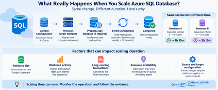
One of the advantages of Azure SQL Database is the ability to scale compute resources without managing the underlying infrastructure. Changing from 4 vCores to 8 vCores can be only a few clicks or a single command. But there is a question I frequently see when troubleshooting scaling operations: "Why is my Azure SQL Database scaling operation taking so long?" An even more interesting question appears when two databases undergo what looks like the same change: Database A Business Critical → Business Critical Scaling duration: ~1 hour 15 minutes Database B Business Critical → Business Critical Scaling duration: ~2 hours 15 minutes Same service tier. Similar scaling request. Very different completion time. At first glance, that might look unusual. However, a scale operation isn't simply Azure changing a configuration value from one number of vCores to another. Depending on the source and target configuration, Azure SQL Database can need to provision target compute, prepare or copy database data, transition connections to the target compute, and clean up the original environment. Microsoft specifically notes that creating a database replica on the new compute instance for some scaling combinations can strongly influence the overall latency. Let's look at what happens and, more importantly, how to monitor it. Scaling Is More Than Changing vCores When you submit a scaling request such as: Business Critical 4 vCores ↓ Business Critical 8 vCores it's tempting to imagine something like: CPU allocation: 4 → 8 Done. That isn't necessarily what happens. At a high level, Microsoft documents a scaling workflow involving two important stages: Create a new compute instance with the requested service tier and compute size Switch routing from the original compute instance to the new one For some combinations of service-tier and compute-size changes, Azure SQL Database must also create a replica on the new compute instance, involving data copying. A simplified view is: Scaling request ↓ Prepare target compute ↓ Prepare/copy database if required ↓ Bring target environment ready ↓ Switch connections ↓ Scaling complete The important takeaway is: A scale operation can involve moving database execution to a new compute environment, not simply increasing CPU on the existing environment. Why Can Two Similar Databases Take Different Amounts of Time? This is where troubleshooting becomes interesting. Imagine two databases: Database A 4 vCores → 8 vCores Completed in 75 minutes Database B 4 vCores → 8 vCores Completed in 135 minutes The natural question is: "If the source and destination configurations are the same, shouldn't the duration also be the same?" Not necessarily. The requested configuration tells us where the database needs to end up. It does not mean the work required to reach that state is identical. Several factors can affect the operation. 1. Database Size and Data Movement One of the most important factors can be the amount of data that must be prepared on the target compute. Microsoft's scaling documentation explicitly states that for some source/target combinations, a replica must be created on the new compute instance. That involves copying data and can significantly affect the overall scaling latency. Conceptually: Small database Provision ████ Data preparation ██████ Switch █ versus: Large database Provision ████ Data preparation ████████████████████████ Switch █ Database size alone doesn't provide a precise prediction of completion time, but it can influence the amount of work required during applicable scaling paths. 2. Workload Activity Matters A database also doesn't necessarily stop processing application traffic while Azure prepares the target environment. Microsoft states that during target compute creation, the database remains online and connections continue to the original compute instance. That creates an interesting challenge: Target environment preparing + Application still generating workload A highly active transactional database and a relatively idle database can therefore present different operational conditions during scaling. The practical lesson is: Two databases with the same service objective aren't necessarily in the same workload state when scaling begins. When investigating a slow scale operation, look at the activity around the scaling window, including: transaction volume; write activity; long-running transactions; workload peaks; batch operations; maintenance activity. 3. Long-Running Transactions Can Affect Switchover Toward the end of scaling, connections need to transition to the target compute instance. Microsoft documents that existing connections to the original compute are dropped and new connections are established to the target compute. The switch generally results in a short interruption, often only a few seconds and generally less than 30 seconds. However, there's an important exception. Microsoft notes that: If long-running transactions are active when connections are dropped, the switch can take longer because aborted transactions need to recover. Conceptually: Normal transition Target ready ↓ Switch ↓ Reconnect ↓ Done With a long-running transaction: Target ready ↓ Connection transition ↓ Transaction interruption ↓ Recovery work ↓ Reconnect ↓ Done This is one reason application workload should be considered when evaluating scaling duration. 4. Resource Availability Can Matter Another clue comes from Azure SQL's operation-status metadata. The sys.dm_operation_status DMV exposes several states for database operations, including: PENDING IN_PROGRESS COMPLETED FAILED CANCEL_IN_PROGRESS CANCELLED Importantly, Microsoft defines PENDING as an operation waiting for resource or quota availability. That means some of the elapsed time around an operation may occur before active processing progresses as expected. This is why comparing scale operations purely by database size or vCore count can be misleading. How Can I Monitor a Scaling Operation? Rather than repeatedly refreshing the Azure portal, there are several useful methods for inspecting progress. Method 1: Azure PowerShell with Get-AzSqlDatabaseActivity Azure PowerShell provides: Get-AzSqlDatabaseActivity Microsoft documents this cmdlet specifically for retrieving the status of operations against Azure SQL databases. For example: Get-AzSqlDatabaseActivity ` -ResourceGroupName "MyResourceGroup" ` -ServerName "myserver" ` -DatabaseName "mydatabase" This can help identify database operations associated with the selected database. For clearer output: Get-AzSqlDatabaseActivity ` -ResourceGroupName "MyResourceGroup" ` -ServerName "myserver" ` -DatabaseName "mydatabase" | Select-Object ` Operation, OperationId, DatabaseName, State, PercentComplete, StartTime, ErrorCode, ErrorMessage The specific fields returned can vary with module/API behavior, so always interpret them in the context of the operation being monitored. The important point is that you're no longer asking only: "Is scaling still happening?" You can inspect the operation itself. Method 2: Check Current and Requested Service Objectives Another useful PowerShell command is: Get-AzSqlDatabase Microsoft documents this cmdlet for retrieving Azure SQL Database properties. Its output includes service-objective information such as CurrentServiceObjectiveName and RequestedServiceObjectiveName. For example: Get-AzSqlDatabase ` -ResourceGroupName "MyResourceGroup" ` -ServerName "myserver" ` -DatabaseName "mydatabase" | Select-Object ` DatabaseName, Status, Edition, CurrentServiceObjectiveName, RequestedServiceObjectiveName During a change, comparing these fields can help establish the current and requested configuration. Think of it as: CurrentServiceObjectiveName ↓ Where am I now? RequestedServiceObjectiveName ↓ Where am I trying to go? Once the operation completes successfully, the current configuration should reflect the requested target. Method 3: Use sys.dm_operation_status For SQL-side monitoring, sys.dm_operation_status provides information about database operations such as CREATE and ALTER. For example: SELECT major_resource_id, operation, state_desc, percent_complete, start_time, last_modify_time, error_code, error_desc FROM sys.dm_operation_status ORDER BY start_time DESC; Useful columns include: operation state_desc percent_complete start_time last_modify_time error_code error_desc Microsoft defines the operation states as including PENDING, IN_PROGRESS, COMPLETED, and FAILED. Be Careful With PercentComplete This is an important detail. It is tempting to interpret: PercentComplete = 50 as: "Half of the work is finished, so half of the remaining time is left." That isn't necessarily correct. For sys.dm_operation_status, Microsoft documents percent_complete for most operations as: 0 = Operation not started 50 = Operation in progress 100 = Operation complete Restore operations are an important exception, where values between 1 and 99 can indicate more granular progress. So for a normal ALTER/scale operation: 50% should generally be interpreted as: The operation is in progress rather than: Exactly half the work remains. This distinction is very useful when communicating with application teams during long-running operations. A Practical Monitoring Script For PowerShell users, I like combining the configuration and operation views. First check the database: $db = Get-AzSqlDatabase ` -ResourceGroupName "MyResourceGroup" ` -ServerName "myserver" ` -DatabaseName "mydatabase" $db | Select-Object ` DatabaseName, Status, Edition, CurrentServiceObjectiveName, RequestedServiceObjectiveName Then check database operations: Get-AzSqlDatabaseActivity ` -ResourceGroupName "MyResourceGroup" ` -ServerName "myserver" ` -DatabaseName "mydatabase" This gives you two complementary perspectives: DATABASE STATE + OPERATION STATE ↓ Better understanding of scaling progress What About Application Availability During Scaling? One of the biggest concerns is: "Does the database remain available while scaling?" For Azure SQL Database, Microsoft states that the database remains online while the new compute environment is being prepared. Connections continue to the original compute during that stage. The important availability event occurs during the transition. At switchover: Existing connections ↓ Dropped ↓ Routing switches ↓ New connections ↓ Target compute Microsoft says the switch generally causes an interruption of less than 30 seconds and often only a few seconds. Applications should therefore implement appropriate transient-error handling and retry logic. Microsoft explicitly recommends retry logic for applications and components using the database while the service tier is being changed. Don't Immediately Cancel a "Slow" Scaling Operation A scale operation taking longer than expected does not automatically mean: Scaling is stuck. It could still be legitimately working through: Resource availability ↓ Target compute preparation ↓ Data/replica preparation ↓ Synchronization / workload handling ↓ Switchover Before assuming failure, gather evidence. Check: Operation state Current service objective Requested service objective Start time Last modification time Error details Workload activity Long-running transactions Then determine whether the operation is: Pending Actively progressing Completed or: Failed Troubleshooting Two Databases With Different Scaling Durations Suppose you're investigating: Database A Scale duration: 1h15 Database B Scale duration: 2h15 Here is the approach I recommend. 1. Verify that the changes truly match Compare: Source service tier Target service tier Source vCores Target vCores Compute tier Storage configuration Do not assume both operations were identical simply because both ended at, for example, Business Critical 8 vCores. 2. Compare database characteristics Look at: Database size Workload level Write activity Transaction volume Long-running transactions 3. Compare operation timing Retrieve: Start time State Last modification time Completion time sys.dm_operation_status exposes this operation metadata for Azure SQL database operations. 4. Determine whether either operation spent time pending Remember: PENDING can mean the operation is waiting for resource or quota availability. That represents a very different explanation from: "The database took longer to copy." 5. Check workload around the transition Look for: Large transactions Bulk writes ETL operations Maintenance High transaction rates Long-running transactions particularly around the switchover period. Scaling Duration Is Not an SLA Stopwatch This leads to perhaps the most important takeaway. If: Database A took 75 minutes you should not assume: Database B must take approximately 75 minutes. Even apparently similar scale operations can encounter different database and platform conditions. A better operational expectation is: Treat each scaling operation as an asynchronous platform operation whose duration depends on the work required to safely reach the requested configuration. Monitor the operation rather than predicting its completion from a previous database. Recommended Checklist Before scaling a production Azure SQL Database: Before Review workload activity. Identify long-running transactions or batch processes. Confirm the requested service objective. Ensure application retry logic is implemented. Record the UTC start time. Understand dependent application connection behavior. During Monitor: Get-AzSqlDatabaseActivity Get-AzSqlDatabase sys.dm_operation_status and watch: State CurrentServiceObjectiveName RequestedServiceObjectiveName StartTime LastModifyTime Error information After Confirm: Current service objective = requested target Database status = Online Application connectivity = Healthy Workload performance = Expected Also validate that applications successfully reconnected after the transition. Final Thoughts When Azure SQL Database scaling takes longer than expected, it's easy to think: "Something must be wrong." And when two similar databases take very different amounts of time, it's equally tempting to expect the durations to match. But a scale operation can involve substantially more than changing a vCore number. At a high level: Request scaling ↓ Provision target compute ↓ Prepare/copy database when required ↓ Transition connections ↓ Complete Microsoft's documentation confirms that data copying for applicable scale paths can strongly influence latency, that the switchover can take longer in the presence of long-running transactions, and that a pending operation might be waiting for resource or quota availability. So when someone asks: "Why is Azure SQL scaling taking so long?" my recommendation is not to start by guessing how many minutes it should take. Instead ask: "What state is the operation currently in, and what evidence do we have about its progress?" With Get-AzSqlDatabaseActivity, Get-AzSqlDatabase, and sys.dm_operation_status, you can turn an opaque waiting period into a much more structured investigation. References Scale single database resources in Azure SQL Database Scale resources in Azure SQL Database sys.dm_operation_status Get-AzSqlDatabaseActivity Get-AzSqlDatabase
Mohamed_Baioumy_MSFT
Oct 16, 2026 Place Azure Database Support Blog
Views
0likes
Comments
Lessons Learned #560: SQL Is Slow — What Can Query Store and SSMS Copilot Uncover?
In our recently delivered session, “SQL Is Slow — What Can Query Store and SSMS Copilot Uncover?”, we demonstrated step by step how to investigate a performance problem by combining Query Store with Copilot’s capabilities in SSMS. The demonstration starts with a PHP program executing queries while we grow a table from a few hundred to millions of rows. As different execution plans appear and performance changes, we follow the evidence in Query Store to uncover what is happening and decide what to investigate next. One clue stood out. The query took about 12 milliseconds per execution in one interval and almost 2.5 seconds in another interval under the same Plan ID. Other plans appeared during the complete lab. Understanding both the differences between plans and the changes within a plan became part of the investigation. Along the way, we demonstrated how a guided conversation with Copilot can become an Agent investigation, and how the investigation itself can be captured in a reusable skill. The useful result was a method that keeps asking for evidence before accepting an explanation. The session brings the two tools together: Query Store supplies the recorded history, and Copilot helps us examine it and decide what to investigate next. The same troubleshooting story lets the audience follow Ask mode, Agent mode and the reusable skill without losing the connection to the underlying SQL evidence. A growing table and several execution plans For our sessions, we use a PHP program that generates 16 different simulations of performance and connectivity problems, allowing us to demonstrate how to investigate these scenarios through practical demos. We also have code developed in .NET and Java. In this demonstration, we add records to dbo.Notes in stages, reaching approximately 200, 32,000, 65,000, 2 million, and 4 million rows, while the PHP program executes dbo.GiveNotes with different @N values. This lets us observe how performance and execution plans evolve as the data volume grows. Several execution plans accumulated during the complete demonstration. We compared all of them, then inspected the runtime intervals within each Plan ID. The reference run revealed this change within the history of one plan: Average per execution Healthy interval Degraded interval Approximate increase CPU 7.69 ms 1,443.19 ms 188 times Duration 12.39 ms 2,473.68 ms 200 times Logical reads 68.39 12,233.10 179 times The duration increase was approximately 200 times. This comparison covers two intervals for one Plan ID, not the whole sequence of table sizes. It does not assign a particular plan or timing to each row-count stage. These are lab observations; identifiers and timings vary between runs. The reads were particularly revealing. Each execution was touching far more pages. A later plan change could not, by itself, explain degradation that had already started while the earlier plan remained in use. The next step was to investigate what had increased the work per execution. Build the timeline before choosing the explanation We first compared workload contributors using total CPU, elapsed duration, logical reads and execution count. Total consumption identified where the workload impact was concentrated; averages per execution helped distinguish expensive executions from a high volume of individually inexpensive calls. Next, we collected every plan for the selected query and compared runtime intervals chronologically. We discovered the identifiers from the database instead of supplying fixed Query IDs or Plan IDs. We asked both when another plan appeared and whether the cost had already increased before that change. A plan summary alone can hide this story. One average across a plan’s entire history blends its healthy and degraded periods. The interval history shows when the work changed and whether that happened before another plan appeared. Aggregation mattered. When combining runtime statistics, we weighted each average by its execution count. A simple average of interval averages would give a lightly used interval the same influence as a heavily used one. We also kept units explicit and separated execution types where needed. Weighted average = SUM(average value * execution count) / SUM(execution count) The increase in logical reads directed the investigation toward the amount of data processed and the access path. Waits could help explain elapsed time, but waits alone would not explain that increase in reads. dbo.GiveNotes filtered dbo.Notes on ID < @N and grouped by Name. The clustered primary key was on id2, a different column from the predicate. As rows were added, a reused plan could process more data; changing @N could also change how many rows qualified. A new Plan ID was a separate event to investigate, not an explanation to assume. Different @N values can qualify different numbers of rows, and table growth can increase the work even with an unchanged plan. We inspected distribution, statistics and access paths to test that explanation. Query Store interval averages alone do not tell us the parameter used by every execution, and parameter-sensitive behavior does not automatically prove parameter sniffing. One investigation through three Copilot experiences In Ask mode, we guided the conversation one question at a time. We first requested the Query Store overview, then asked which contributor to investigate and how its plans behaved over time. The staged prompts delayed statistics, index and parameter analysis until the runtime evidence justified those questions. Where required, we ran generated diagnostic T-SQL and brought the results back into the conversation. In Agent mode, we supplied the investigation goal and allowed Copilot to choose and execute diagnostic steps using the available SQL tools. We reviewed the proposed actions and kept the investigation read-only. The agent could use each result to decide what to inspect next. Finally, we captured the sequence in an Agent Skill. We wanted the next investigation to preserve the critical question: did the query become more expensive while the same plan was still being reused? Agent Skills provide task-specific instructions that Copilot can discover and use in Agent mode. We also demonstrated the reusable method through GitHub Copilot CLI. Database execution still requires a configured SQL tool or MCP server; without that capability, the workflow must generate diagnostics for the engineer to run. What we put into the reusable skill The SQL Performance Investigator pack captures the diagnostic sequence alongside the calculation rules and starting prompts. The agent is instructed to: Identify the main workload contributor and retain its Query ID. Collect all associated plans and their runtime history. Check whether degradation began while the same plan remained in use. Investigate relevant selectivity, statistics and index evidence. Separate confirmed observations from hypotheses and propose validation. A skill makes the method reusable; it does not guarantee the diagnosis is correct. Missing history, incorrect aggregation or a plausible but unsupported inference still need an engineer’s attention. We kept discovery read-only, with SQL permissions enforcing the access boundary. A proposed index still needs evidence of improvement In the demonstration, we evaluated an index with ID as its leading key and Name as an included column: CREATE NONCLUSTERED INDEX NOTES_IX1 ON dbo.Notes (ID) INCLUDE (Name); The key matches the range predicate, while the included column makes Name available for the aggregation. Whether this improves the workload depends on selectivity, data volume and the competing plans. Its storage and write costs also matter. We treated this as a remediation candidate. Validation requires a comparable workload, including parameter distribution and concurrency, followed by a Query Store comparison of reads, CPU, duration and variability. We did not equate an index recommendation with a demonstrated improvement. Statistics also need careful interpretation. An index histogram describes its leading key; adding Name as an INCLUDE column does not create a histogram on Name. An existing auto-created statistic should not be dropped merely because its column appears in a covering index. The lesson we took from the demonstration The complete story contained a growing table and multiple plans. Within that history, one plan became much more expensive before a later plan could explain the change. Comparing plans and examining changes within each plan gave us complementary evidence. Copilot helped us follow it, and the skill preserved the investigation sequence for another database. We enjoyed presenting this session. For DBAs, developers and support engineers, the session offers a practical way to watch a performance investigation unfold, from the PHP workload and Query Store history to the prompts and reusable skill. We look forward to continuing this demonstration and discussion with SQL user groups and the wider technical community. If you have encountered a query that became slower while the same plan remained in use, which evidence helped you explain the change? We would be interested to hear how you approached it. References and prerequisites For the SSMS Agent and Skills experience described here, Microsoft documents SSMS 22.7 or later with the AI Assistance workload and GitHub Copilot access. Query Store must be enabled with relevant history available. Specify the target server and database in the Agent prompt rather than relying on the active editor context. Check the current documentation before reproducing the session. GitHub Copilot Agent mode in SSMS Agent Skills in SSMS Monitoring performance by using Query Store Query Store runtime statistics Try the investigation with our prompts These prompts offer a practical starting point for the method demonstrated in our session. The Ask prompt is the opening prompt from our session workflow. The Agent prompts are adapted from our accompanying pack to make the target server, database and investigation window explicit. Replace the angle-bracket placeholders before submitting them. Start with Ask mode We began with a request for evidence, deliberately postponing diagnosis. Run the generated diagnostic query against the intended lab database and use its results for the next questions. I want to start a SQL performance troubleshooting investigation using Query Store. Generate a single read-only T-SQL query that I can execute in the current database to identify the main performance contributors. The query must use Query Store and return, for each query: * Query ID * Query text * Object or stored procedure name, when available * Number of execution plans * Number of executions * Total CPU time * Average CPU time per execution * Total duration * Average duration per execution * Total logical reads * Average logical reads per execution Aggregate Query Store runtime statistics correctly across runtime intervals and execution plans. Use weighted calculations based on count_executions. Do not calculate averages by simply averaging Query Store average values. Return CPU and duration values in milliseconds. Rank the results by total CPU consumption, but include all the metrics above so that we can determine later which resource is having the highest impact. Do not perform root-cause analysis yet. Do not include execution plan analysis, parameter sensitivity, statistics analysis, index analysis, or remediation recommendations. Only generate the read-only diagnostic T-SQL query that I should execute. We then asked which resource deserved investigation, which query contributed most, how all its plans performed over time, and whether the same Plan ID had become more expensive. Only after those answers did we investigate selectivity, statistics and indexes. The complete session workflow contains the staged follow-up prompts. Convert the conversation into an Agent investigation We moved the recurring calculation rules and diagnostic sequence into sql-performance-investigator. The starting prompt could then state the goal, scope and execution boundaries. The skill supplies the detailed method; the available SQL tools supply execution capability. The agent retains the discovered query and plan identifiers within the investigation. It should not ask the engineer to copy them between steps or assume the identifiers from a previous lab run. Run the method in SSMS Agent mode Make the skill available to SSMS, select Agent mode and verify the SQL tools are enabled. Specify the target explicitly because Agent mode does not inherit the active query editor context. Investigate the SQL performance problem on server <server>, database <database>, using Query Store for <UTC start> to <UTC end>. Use the sql-performance-investigator skill. Use the available sql-tools to execute read-only diagnostics and continue through the investigation, requesting approval where the host requires it. Automatically discover the dominant performance metric, target query, Query ID, all Plan IDs, runtime history, and any same-plan degradation. Retain the discovered identifiers internally. Investigate the evidence needed to explain the change, including selectivity, data distribution, statistics and existing indexes when relevant. Do not assume a plan change caused the degradation or label it parameter sniffing without evidence. Keep confirmed evidence, inference, hypotheses and missing evidence separate. Use execution-weighted averages and explicit units. If the requested history or permissions are unavailable, report the limitation. Do not create/drop indexes, update/drop statistics, force plans, clear caches, modify Query Store, or change data/schema. Finish with a supported diagnosis or remaining uncertainty, a proposed remediation if justified, and a Query Store before/after validation plan. Do not execute remediation. Use the same method in GitHub Copilot Our pack places the skill at .github/skills/sql-performance-investigator/SKILL.md and the Custom Agent at .github/agents/sql-performance-investigator.agent.md. The skill references workflow.md and query-store-rules.md for the detailed method. In GitHub Copilot CLI, select the SQL Performance Investigator custom agent and use this adapted starting prompt: Use the SQL Performance Investigator custom agent and the sql-performance-investigator skill. Investigate SQL performance on <server>, database <database>, for <UTC start> to <UTC end>, using Query Store from evidence to diagnosis. If a SQL execution tool/MCP is available, run only read-only diagnostics and continue through the investigation. Discover Query IDs and Plan IDs automatically and retain them internally. Follow the host approval requirements. If no SQL execution capability is available, generate one self-contained read-only diagnostic batch for me to run, then continue when I provide the result. Do not claim that SQL was executed. Do not apply remediation. Propose an index/statistics action only after the evidence supports it. Finish with a before/after Query Store validation plan. The reusable asset is the investigation procedure behind these prompts. Query Store supplies the evidence, Copilot helps carry out the investigation, and the engineer reviews whether the explanation and proposed change are supported by the results.
Jose_Manuel_Jurado
Oct 16, 2026 Place Azure Database Support Blog
Views
0likes
Comments
Azure SQL Performance Troubleshooting: When High Latency Is Not High CPU
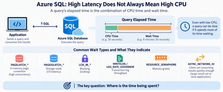
When an application connected to Azure SQL Database becomes slow or starts timing out, one of the first questions is usually: Is the database running out of CPU? It's a reasonable starting point, but CPU is only one part of the performance story. Some Azure SQL performance problems occur while CPU, Data IO, and worker utilization appear healthy. The database may have plenty of compute capacity while queries spend most of their time waiting rather than executing. The key troubleshooting question is therefore not simply: "How much CPU is Azure SQL using?" Instead, ask: "Where is the elapsed time being spent?" Start With Resources, But Don't Stop There Resource utilization should still be the first checkpoint. A simple query using sys.dm_db_resource_stats can help identify whether Azure SQL is approaching CPU, Data IO, Log IO, memory, or worker limits: SELECT DB_NAME() AS database_name, AVG(avg_cpu_percent) AS avg_cpu_percent, MAX(avg_cpu_percent) AS max_cpu_percent, MAX(avg_data_io_percent) AS max_data_io_percent, MAX(avg_log_write_percent) AS max_log_write_percent, MAX(avg_memory_usage_percent) AS max_memory_percent, MAX(max_worker_percent) AS max_worker_percent FROM sys.dm_db_resource_stats; If CPU is consistently near 100%, investigate CPU consumption. If Log IO reaches its limit, investigate transaction-log generation. If workers are exhausted, investigate concurrency. But if none of these resources is saturated, don't conclude that Azure SQL is healthy. Move to wait analysis. Follow the Waits A useful simplified model is: Query elapsed time = CPU execution If a query runs for 10 minutes but uses only 30 seconds of CPU, most of its elapsed time occurred somewhere else. Common wait patterns can point the investigation in different directions: Wait Area to investigate PAGELATCH_* In-memory page contention PAGEIOLATCH_* Storage reads LCK_M_* Blocking WRITELOG Transaction log LOG_RATE_GOVERNOR Log throughput RESOURCE_SEMAPHORE Memory grants ASYNC_NETWORK_IO Client/result consumption The wait type is not automatically the root cause. Think of it as a sign telling you: Look in this direction next. PAGELATCH Does Not Mean Slow Storage One important distinction is: PAGELATCH versus: PAGEIOLATCH Despite their similar names, they represent different problems. PAGEIOLATCH is associated with waiting for data pages involved in physical I/O. PAGELATCH, however, is synchronization around pages that are already in memory. Consider a highly concurrent workload: Hundreds of sessions ↓ Same memory page ↓ Latch contention ↓ Sessions wait ↓ Application CPU may still have available capacity. This is why increasing vCores doesn't necessarily eliminate latch contention. Additional compute provides more workload headroom, but it doesn't automatically remove a serialization point around a hot page. Microsoft's I/O troubleshooting guidance also distinguishes PAGEIOLATCH and other I/O-related waits when diagnosing storage-performance problems. Microsoft Learn: Troubleshoot SQL Server I/O performance Query Frequency Matters Too Another common mistake is focusing only on individually expensive queries. Imagine a query that takes only 20 milliseconds but executes hundreds of thousands of times, often concurrently. Its impact is better thought of as: Workload Impact = Cost per execution × Execution frequency × A small metadata lookup or initialization query can become significant when hundreds of application instances execute it simultaneously. This is where Query Store becomes particularly useful. Query Store preserves query, execution-plan, and runtime history, allowing you to compare executions, duration, CPU, plans, and other performance characteristics over time. Microsoft Learn: Monitor performance using Query Store Instead of asking only: "What's my most expensive query?" also ask: "What changed in the workload?" When Nine Hours of Duration Is Only One Minute of CPU Now consider the opposite problem. Suppose Query Store shows something like: Elapsed time 9 hours SQL CPU time 1 minute Returned rows 750,000+ Dominant wait ASYNC_NETWORK_IO Would adding CPU solve this? Probably not. CPU represents only a tiny fraction of the elapsed time. ASYNC_NETWORK_IO commonly occurs when SQL Server has results available but the client application is not consuming them quickly enough. Microsoft documents several possible causes, including: large result sets; slow application processing; applications fetching rows slowly; network-related delays. Microsoft Learn: Troubleshoot ASYNC_NETWORK_IO Importantly: ASYNC_NETWORK_IO does not automatically mean the network is slow. The bottleneck might actually be the application. Measure Time to First Row A useful troubleshooting technique is to separate database response time from result-consumption time. Instead of measuring only: Query start → Application finished measure: T0 = Query submitted T1 = First row received T2 = Last row received T3 = Application processing completed You can then separate: Database response = T1 - T0 Result consumption = T2 - T1 Application For example: First row received: 2 seconds Last row received: 2 hours Processing completed: 2.5 hours Calling this a "2.5-hour SQL query" would be misleading. SQL started returning results after two seconds. Most of the time was spent transferring or processing them. Don't Forget Blocking Low CPU can also be caused by blocking. If many sessions are waiting behind a transaction, increasing CPU isn't going to solve the problem. During an active incident, check requests and their waits: SELECT r.session_id, r.blocking_session_id, r.status, r.wait_type, r.wait_time, r.wait_resource, r.cpu_time, r.total_elapsed_time, st.text FROM sys.dm_exec_requests AS r CROSS APPLY sys.dm_exec_sql_text(r.sql_handle) AS st WHERE r.blocking_session_id <> 0 ORDER BY r.wait_time DESC; This helps determine whether the application is experiencing a resource problem or simply waiting behind another transaction. Why Scaling Can Be Misleading Imagine this sequence: Application slow ↓ Scale database ↓ Performance improves It's tempting to conclude: "We needed more CPU." But scaling can change more than CPU availability. Depending on the operation and environment, it can alter resource availability or execution conditions. Therefore: A successful mitigation does not automatically prove the root cause. Always distinguish between: What made the symptoms disappear? and: What originally caused the symptoms? A Practical Troubleshooting Workflow When investigating Azure SQL performance, I use the following approach: 1. Define the exact incident window Preferably using UTC timestamps. 2. Check core resources Look at: CPU Data IO Log IO memory workers 3. Compare CPU time with elapsed time If: Elapsed ≈ CPU investigate computational workload. If: Elapsed >>> CPU investigate waits. 4. Identify dominant waits Ask what prevented SQL from continuing execution. 5. Check blocking Determine whether requests are waiting behind other transactions. 6. Use Query Store Compare healthy and problematic periods for: execution count; CPU; duration; logical reads; plans; wait behavior. Microsoft provides Query Store examples specifically for workload and performance investigation. Microsoft Learn: Tune performance with Query Store 7. Inspect the execution plan Look for inefficient access patterns, cardinality problems, excessive reads, repeated lookups, spills, scans, or plan changes. 8. Investigate the application Especially when SQL CPU is low but result-transfer waits are high. Look at: rows returned; fetch size; batch size; application processing; concurrency; downstream dependencies. 9. Compare healthy vs unhealthy periods Don't analyze an incident in isolation. Ask: What changed? Common Misdiagnoses "CPU isn't 100%, so SQL is healthy." Not necessarily. Queries might simply be waiting. "ASYNC_NETWORK_IO means we have a network problem." Not necessarily. The client may be consuming results slowly. "PAGELATCH means storage is slow." No. Don't confuse PAGELATCH with PAGEIOLATCH. "Scaling fixed the problem, so CPU was the root cause." Not necessarily. Mitigation and root cause are different concepts. "The slowest query must be the problem." Not always. A small query executed extremely frequently can generate larger cumulative impact. Final Thought: Follow the Time When Azure SQL becomes slow, avoid jumping directly from: Slow database → Add more vCores Instead, work through: High latency ↓ Resource utilization ↓ CPU vs elapsed time ↓ Wait statistics ↓ Query Store ↓ Execution plan ↓ Application behavior ↓ Root cause ↓ Targeted optimization Performance troubleshooting becomes much easier once you stop asking only: "How busy is Azure SQL?" and start asking: "Where did the time go?" Because sometimes the database isn't busy at all. It's waiting. References Monitor Performance by Using the Query Store Tune performance with the Query Store Troubleshoot slow queries resulting from ASYNC_NETWORK_IO Troubleshoot slow SQL Server performance caused by I/O issues
Mohamed_Baioumy_MSFT
Oct 16, 2026 Place Azure Database Support Blog
Views
0likes
Comments
Lessons Learned #559: Understanding query timeouts in Azure SQL Database
In a recent support case, an application using Hibernate and the Microsoft JDBC Driver for SQL Server reported "The query has timed out". The application team had timestamps for the failures, but the SQL evidence reviewed did not show matching query cancellations. This raised a question that developers and DBAs frequently ask: If the exception contains SQLServerException, does that mean the database engine generated the timeout? The important distinction is where the timeout is reported and enforced, versus what caused the operation to exceed that limit. A command timeout is controlled by the client. Its underlying cause can still be a slow query, blocking, a communication delay, or another issue along the client and database path. In this article, we will explain that distinction, what to capture when it happens, and when increasing the command timeout can be appropriate. The examples use invented values and generic statements; no customer identifiers or application SQL are included. First identify which timeout occurred An application request can wait at several different stages. Before changing a setting, identify the stage that failed. Stage What to check Acquiring a connection from the pool Pool capacity, connection lifetime, and the pool acquisition timeout Establishing a database connection Connection or login timeout, endpoint, authentication, and handshake evidence Executing a SQL command Effective JDBC query timeout or SqlClient CommandTimeout, query execution, and blocking Communicating with the server Driver socket settings and evidence of interrupted or delayed communication Processing the application request ORM processing and the application's request or transaction deadline Changing a connection timeout does not increase the query timeout. Similarly, an HTTP request deadline is not the same setting as a database command timeout. A failure while obtaining a pooled connection should not automatically be investigated as a query that timed out in SQL. The Microsoft JDBC timeout documentation distinguishes these settings. JDBC queryTimeout and cancelQueryTimeout use seconds; socketTimeout uses milliseconds. Understand what the exception tells us The useful part of the exception chain in this case was: org.hibernate.QueryTimeoutException Caused by: java.sql.SQLTimeoutException: The query has timed out. Caused by: com.microsoft.sqlserver.jdbc.SQLServerException: The query has timed out. ... TDSCommand.checkForInterrupt(...) The stack places the observed exception in the client/JDBC execution and response handling path, propagated through Hibernate. SQLServerException is a driver exception class. Its presence alone does not establish that SQL Server generated a corresponding engine error. This is a client reported query timeout. That describes the observed error, not the root cause. If blocking prevents a command from completing before the client's limit, the client raises the timeout, while the delay is explained by database activity. Developers and DBAs need to investigate the same attempt together. What queryTimeout actually controls The Microsoft JDBC Driver uses queryTimeout to limit its wait for a server response after sending an execute command. When that timeout expires, the documented behavior is to cancel the command. cancelQueryTimeout controls the subsequent wait for acknowledgment of cancellation before the driver closes the connection. These settings do not define an exact stopwatch for the entire business request. Pool acquisition, connection establishment, cancellation handling, retries, and application processing can have different deadlines. The caller's total elapsed time can therefore differ from the configured query timeout. For JDBC, setQueryTimeout sets the timeout on a statement in seconds. In .NET, the corresponding setting is SqlCommand.CommandTimeout. Its documented semantics include network reads during command execution or result processing; it is not a limit on all user code that processes those results. The default is also provider dependent. SqlClient documents a 30 second default. Do not assume the same default for JDBC or for statements created by an ORM. Check the effective value used by the failing operation. This client command timeout is not an Azure SQL Database engine configuration setting. The same distinction applies when the application connects to Azure SQL Managed Instance or SQL Server on an Azure VM. How a command timeout becomes an Attention The application configures the driver's deadline; it does not send a "CommandTimeout" SQL error to the engine. The diagram shows the cancellation path for a request already sent through the Microsoft JDBC Driver. If the command completes within the limit, no timeout driven Attention is needed. Figure 1. The application owns the deadline. The driver enforces it and requests cancellation; the engine handles the SQL request. The values are illustrative, not recommended settings. For an already submitted request, Attention is a TDS cancellation message. SQL Server marks the request for cancellation and honors it at yield points, as described in the Attention and error 3617 guidance. The timer expiring and the engine stopping are not necessarily simultaneous. The driver consumes the remaining response until it receives the cancellation acknowledgment. The TDS cancellation state describes this response cleanup. A query timeout normally leaves the connection open after that exchange; it does not immediately cut off all communication. If no acknowledgment arrives and a configured cancelQueryTimeout expires, the Microsoft JDBC Driver closes the connection. A socket timeout or transport failure can also close it. Closing the socket alone does not establish the SQL operation's outcome. Other providers can have different cancellation and connection handling details. What we could conclude from the case We reviewed the reported failure windows, the available SQL activity, and the query identified by the application team. Some client initiated aborts were recorded, but we could not correlate them with the reported failures. The resource metrics reviewed did not establish resource pressure as the cause either. The supported conclusion was that the client reported a query timeout, while the SQL evidence reviewed did not identify a matching cancellation or establish the root cause. Further correlation was required. The reported statement was a SELECT. The transaction and write examples later in this article explain additional design considerations; they are not findings of failed writes or abandoned transactions in this case. Statistics maintenance had also been performed, but that action did not establish why the client timed out. A fast maximum or average in the available query statistics does not prove that the failed attempt was fast. Confirm the query, parameter types, destination database and replica, execution context, and time window. Successful executions and retries may appear alongside the attempt that failed. Developers should capture each failed attempt The message alone is not enough. Record the failure as an individual attempt that a DBA can correlate with database evidence. Evidence to record Why it matters UTC start and error timestamps and elapsed time Establish the failure window and observed duration Request correlation identifier and attempt number Separate the original call from retries Full exception chain and available SQLState or error code Identify the provider and phase reporting the failure Driver and ORM versions and effective timeout with its unit Establish which settings actually applied Parameterized SQL template and parameter types Identify the statement without publishing customer data Protected destination and connection identifiers Correlate with the correct database, replica, and session Measure pool acquisition, execution, result reading, and subsequent application processing separately. A request duration alone cannot tell us where the time was spent. If the ordinary logs are insufficient, collect a targeted JDBC driver trace during the same window. Keep credentials and personal data out of diagnostic examples. Retain the necessary correlation details in controlled diagnostic records and anonymize them before sharing publicly. DBAs should correlate cancellations with execution evidence On the database side, use Extended Events to capture sqlserver.attention together with relevant batch or RPC start and completion events. Correlate the timestamps and session or connection information with the application's failed attempt. The query timeout troubleshooting guidance describes this approach. An Attention indicates a client cancellation signal, but it does not identify why the client canceled. A user pressing Cancel can also produce it. Compare the associated execution duration with the application's effective timeout and logs; do not interpret the Attention event's own duration as the query's total runtime. Query Store adds historical context. In sys.query_store_runtime_stats, execution_type = 3 means client initiated aborted execution. It is not an exclusive count of query timeouts. Query Store statistics are aggregated. Select intervals overlapping the incident window, aggregate rows for the same plan, execution type, and interval, and examine both aborted and regular executions. Filtering only on last_execution_time can miss relevant activity within an interval. A query hash identifies a query family, not an individual request. For additional examples, see Lesson Learned 1 on capturing a TSQL command timeout, Lesson Learned 202 on reproducing and finding a command timeout, and Lesson Learned 525 on tracking timeouts beyond Query Store with Extended Events. For Azure SQL Database, use database scoped Extended Events. Check capture coverage, filters, retention, and possible event loss before interpreting missing events. Do not expect every command timeout to appear in the SQL error log. Also check transaction cleanup. Canceling a statement does not guarantee that the entire explicit transaction has been rolled back. The application's error handling must account for the resulting transaction state, as explained in the Azure SQL blocking guidance. When increasing the command timeout makes sense In Lesson Learned 253 and Lesson Learned 372, I shared examples that increase the execution timeout across retry attempts, including a PowerShell example. That technique changes how long the client is prepared to wait. It does not make the SQL statement execute faster. A bounded increase may be appropriate when the workload legitimately needs more time, or as a temporary mitigation while investigating. It can also help a controlled diagnostic execution complete so its behavior can be examined. If the operation normally completes quickly but suddenly exceeds the limit, investigate blocking, plan changes, resource waits, and communication before treating a larger timeout as the permanent solution. Verify the change against representative load and the application's response time requirements. The following examples show where the setting belongs. They assume an already open connection and run a generic statement with an intentional delay. Use them only in a test environment. For Java with the Microsoft JDBC Driver: try (java.sql.Statement statement = connection.createStatement()) { statement.setQueryTimeout(20); // seconds statement.execute("WAITFOR DELAY '00:00:12'; SELECT 1;"); } For .NET with Microsoft.Data.SqlClient: using var command = connection.CreateCommand(); command.CommandTimeout = 20; // seconds command.CommandText = "WAITFOR DELAY '00:00:12'; SELECT 1;"; using var reader = command.ExecuteReader(); With a 5 second command timeout, the deliberate 12 second delay should produce a timeout. With 20 seconds, the operation should have time to complete under normal test conditions. The delay has not become shorter; only the client's permitted wait has changed. This demonstrates the mechanism, not a fix for the original case. For each test, record the UTC start and end, effective timeout, elapsed time, exception, and attempt identifier. Capture Attention and the related execution events at the same time. Compare the two runs: the application setting changed, while the SQL statement and database configuration remained the same. Use the captured events to verify the expected behavior rather than assuming exact timestamps or a fixed event count. When an ORM creates the statement, apply the equivalent setting through the supported ORM configuration and verify its effective value and unit. Setting setQueryTimeout(0) or CommandTimeout = 0 removes that statement's timeout limit; it should not be a routine response to unexplained failures. If retries are used, record the timeout on every attempt, limit the attempts, allow a delay between them, and keep the total within the request's overall deadline. Transactions determine what must succeed or fail together A single UPDATE, INSERT, or DELETE already executes within a transaction in autocommit mode. Use an explicit transaction when several statements form one business operation and must be committed or rolled back together. The transaction documentation describes these transaction modes. For example, an application might UPDATE inventory, INSERT an order, and DELETE its reservation. If the first two statements finish and the third is canceled, the outcome depends on how the unit of work was managed. Transaction design What the application must account for Each statement in autocommit Earlier statements may already be committed. Canceling the later statement does not undo those earlier commits. One explicit transaction for all three statements Earlier changes remain part of that transaction until it is committed or rolled back. An Attention alone does not guarantee rollback of the whole transaction. COMMIT sent but its confirmation not received The client may not know whether the transaction committed. Verify the outcome before retrying the business operation. One transaction preserves the intended unit of work; it does not replace timeout and error handling. An open transaction left after cancellation can retain locks and delay other sessions. A poorly handled timeout can therefore contribute to further timeouts. Keep the transaction as short as the business rules allow. Do not include user interaction or unrelated external calls while holding it open. A command timeout also does not automatically limit the transaction's total duration: if the application sends several commands separately, each command has its own limit. Track the total operation deadline as well. A rollback inside TSQL CATCH may never run for Attention This is an important detail for developers: T-SQL TRY CATCH does not catch Attentions, including client interrupt requests. Placing ROLLBACK only in a stored procedure's CATCH block is therefore insufficient protection against a client cancellation. The application or ORM that owns the transaction must handle the failed call and resolve that transaction. Attempt rollback using its transaction API when the connection remains usable; log cleanup failures separately and do not continue using an unresolved transaction. A rollback attempt is not proof of a completed rollback. Follow the provider's cleanup rules before returning the connection to normal pool use. SET XACT_ABORT ON controls transaction abortion for applicable runtime errors. Microsoft's Attention and transaction guidance also describes it as a way to control rollback when a cancellation occurs. Set it deliberately for the SQL session or batch and validate the behavior with the actual driver, ORM, and transaction ownership model. It does not change CommandTimeout, and it cannot undo a transaction that already committed. In a disposable test environment, repeat the cancellation experiment inside a transaction after a small data modification. Compare XACT_ABORT OFF and ON. After cancellation acknowledgment, inspect transaction state on the same usable connection and ensure cleanup. If cancellation closes the connection, record that outcome instead of claiming to have queried its former session. This test is separate from the original SELECT investigation. A timeout does not establish whether a write committed If a connection fails after COMMIT was processed but before its acknowledgment reaches the application, the client can receive an error even though the changes were committed. Retrying an INSERT or increment blindly can then duplicate a business operation. Microsoft's connection resiliency documentation describes this commit failure and idempotency issue. Use a stable operation identifier that is reused across retries. Record it atomically with the business changes and enforce uniqueness in the database, so a repeated attempt can identify the prior operation rather than apply it again. If the original transaction is still in progress, resolve or wait for its outcome; an absent record in a single check is not always conclusive. The transaction provides atomicity for the changes. An operation identifier and deliberate retry handling help the application manage an uncertain result. Together, they make the timeout response part of the business operation's design.
Jose_Manuel_Jurado
Oct 12, 2026 Place Azure Database Support Blog
Views
0likes
Comments
Lessons Learned #558: What an Execution Plan XML Can Tell Us in Azure SQL Database
During a performance investigation in Azure SQL Database, we requested the execution plan to understand what the query was doing. While reviewing the evidence, the customer asked a broader question: when you open the XML of an execution plan, what do you usually look for? It was a useful question. The graphical plan helps us follow the flow of data, but the XML contains details about parameters, statistics, warnings and execution that can explain why the query behaved as it did. I do not read every attribute. I start with a few checks that help connect the customer symptom to the work performed by the query. In this article, I will walk through those checks: the type of plan, parameter values, estimated versus actual rows and statistics, missing indexes and implicit conversions, and reasons for a serial plan. The XML fragments below are simplified examples that use invented values or are adapted from examples discussed in previous articles in the Lessons Learned troubleshooting series. First check whether the plan contains execution evidence Plan What we can inspect Estimated plan Optimizer choices and estimates; the query has not executed Actual plan Plan plus available counters and warnings from that execution Cached or Query Store plan Compiled plan; normally no operator actuals for the incident For the checks involving actual rows, I request an actual execution plan. In SSMS, use Include Actual Execution Plan, or capture it using SET STATISTICS XML. Choose one method. The latter executes the query and returns its plan. The account needs the permissions to run the statement and SHOWPLAN permission. SET STATISTICS IO ON; SET STATISTICS TIME ON; SET STATISTICS XML ON; -- Execute the SELECT being investigated here. SET STATISTICS XML OFF; SET STATISTICS TIME OFF; SET STATISTICS IO OFF; Save the plan as a .sqlplan file and keep the Messages output. Record when it was captured, the parameters and the reported symptom. An execution captured later may not represent the incident. Review query literals, parameter values and object names before sharing the file. Check the right statement and its parameters A procedure or batch may contain several statements. I locate the relevant StmtSimple and its QueryPlan before interpreting a warning. StatementId and operator NodeId help keep the observations attached to the correct statement and operator; NodeId is not a stable identifier across different compilations. Next, I look at ParameterList. When available, it shows both the value used when the plan was compiled and the value used during the captured execution. <ParameterList> <ColumnReference Column="@CustomerId" ParameterDataType="int" ParameterCompiledValue="(42)" ParameterRuntimeValue="(900)" /> </ParameterList> Here, the plan was compiled with CustomerId 42 and executed with CustomerId 900. If one customer has a few orders and another has thousands, I would compare their data distribution and actual plans. Different values are a reason to investigate parameter sensitivity; they do not prove that plan reuse caused the problem. A missing runtime value means this capture did not provide it. It does not mean the runtime value was the same as the compiled value. Also, eligible queries can intentionally use different plan variants through Parameter Sensitive Plan optimization. Make the comparison match the application If the query is slow in the application but fast in SSMS, I compare the SQL text, parameter types and values, database context and session options. StatementSetOptions records options associated with compilation. <StatementSetOptions ARITHABORT="true" ANSI_WARNINGS="true" ANSI_NULLS="true" QUOTED_IDENTIFIER="true" ANSI_PADDING="true" CONCAT_NULL_YIELDS_NULL="true" NUMERIC_ROUNDABORT="false" /> A difference in context can help explain why the application and SSMS use different cached plans. I capture both rather than assuming that a fast SSMS execution represents the application. The difference itself still needs to be connected to the measured performance. Compare estimated and actual rows then inspect statistics I follow the rows through the plan and look for the first useful difference between what the optimizer expected and what the operator actually processed. <RelOp NodeId="3" PhysicalOp="Index Seek" LogicalOp="Index Seek" EstimateRows="100"> <RunTimeInformation> <RunTimeCountersPerThread Thread="0" ActualRows="20000" ActualRowsRead="80000" ActualExecutions="1" /> </RunTimeInformation>  </RelOp> In this single-execution example, the operator estimated 100 rows and returned 20,000: a 200-fold underestimate. It also read 80,000 rows. I would ask why the estimate was inaccurate, and why the operator read substantially more rows than it returned. These are separate questions. For repeated or parallel operators, account for executions and threads before comparing totals. Do not add the rows from every operator to calculate the query result size. The next question is often whether the statistics were out of date. OptimizerStatsUsage identifies statistics consulted during compilation, where that information is exposed. <OptimizerStatsUsage> <StatisticsInfo Schema="[PlanXmlLab]" Table="[Orders]" Statistics="[IX_Orders_CustomerId]" LastUpdate="2026-10-10T07:00:00" SamplingPercent="20" ModificationCount="15000" /> </OptimizerStatsUsage> I check the relevant statistics object, its LastUpdate, SamplingPercent and ModificationCount together. An old timestamp or a low sampling percentage alone does not prove that it caused the estimate. Updated statistics cannot explain every discrepancy; parameter values, predicates and data distribution also matter. The XML describes the statistics consulted at compilation. To check their current state, I use sys.dm_db_stats_properties, as shown next. A subsequent update does not rewrite the evidence in an already saved plan. Check when the statistics were last updated -- Run in the affected database and set the actual table name. SELECT st.name AS statistics_name, sp.last_updated, sp.rows, sp.rows_sampled, sp.modification_counter FROM sys.stats AS st OUTER APPLY sys.dm_db_stats_properties( st.object_id, st.stats_id) AS sp WHERE st.object_id = OBJECT_ID(N'PlanXmlLab.Orders'); last_updated identifies the latest statistics update; rows and rows_sampled describe the population and sample at that update. modification_counter counts modifications to the leading statistics column since the update. Metadata visibility and permissions can affect the output. Compare this information with the same statistics object in the plan. Timestamps alone do not tell us whether the update was automatic or manual. If an update is justified, validate it in a controlled comparison using the same query and representative parameters, and capture a newly compiled plan. Read the access path alongside the row counts An Index Seek can still read many rows. I inspect SeekPredicates, any residual Predicate and ActualRowsRead where available. A broad seek range followed by filtering can explain why the rows read greatly exceed the rows returned. Likewise, a Key Lookup may be inexpensive once but expensive when repeated for thousands of rows. A scan can be the right choice when a large part of the table qualifies. The operator name is a starting point; the amount of work tells us more. For the customer, the useful explanation is concrete: this operator returned many more rows than expected, these were the statistics used, and this is the next comparison that will help establish why. That is more informative than recommending a statistics update from the timestamp alone. Read missing indexes and conversion warnings as clues Missing-index messages are easy to notice. I inspect the suggestion, but I also check whether it fits the query and the existing indexes. <MissingIndexes> <MissingIndexGroup Impact="85.0"> <MissingIndex Schema="[PlanXmlLab]" Table="[Orders]"> <ColumnGroup Usage="EQUALITY"> <Column Name="[CustomerId]" ColumnId="2" /> </ColumnGroup> <ColumnGroup Usage="INCLUDE"> <Column Name="[Amount]" ColumnId="3" /> </ColumnGroup> </MissingIndex> </MissingIndexGroup> </MissingIndexes> This example suggests a key on CustomerId with Amount included for coverage. EQUALITY and INEQUALITY describe predicate columns, while INCLUDE describes covering columns. The suggestion does not settle every detail of index design. Impact is an estimated reduction in optimizer cost. A value of 85 does not promise an 85% reduction in elapsed time. The XML may contain more suggestions than the graphical plan displays. Review existing indexes and write overhead, then measure the candidate change. Check which side of the predicate is converted <Warnings> <PlanAffectingConvert ConvertIssue="Seek Plan" Expression="CONVERT_IMPLICIT(nvarchar(50),[dbo].[Customers].[Code],0)" /> </Warnings> In this separate example, I would inspect the Code column type and the application parameter declaration. A varchar column compared with an nvarchar parameter can introduce a conversion on the column side because nvarchar has higher type precedence. The warning identifies something that may affect the plan, not a measured root cause. Whether a conversion prevents an efficient seek depends on the types, collation and expression. Test an appropriate parameter declaration while preserving required character semantics, and compare results, reads and CPU. A conversion in the projection is different from one in a search predicate. Look for an explicit reason when the plan is serial Customers sometimes ask why a query does not run in parallel when the database has multiple vCores. I look for NonParallelPlanReason in QueryPlan before assuming that more resources or a higher MAXDOP will change the result. <QueryPlan DegreeOfParallelism="0" NonParallelPlanReason="TSQLUserDefinedFunctionsNotParallelizable">  </QueryPlan> Reason What I inspect next MaxDOPSetToOne Effective MAXDOP setting or query hint TSQLUserDefinedFunctionsNotParallelizable Scalar UDF and its inlining behavior NonParallelizableIntrinsicFunction The specific intrinsic function referenced A serial plan can be appropriate. The attribute can identify a restriction, but its absence does not fully explain the optimizer decision. Scalar UDF inlining can remove a restriction without guaranteeing parallel execution. DegreeOfParallelism="1" does not demonstrate parallel work. In Azure SQL Database, check database-scoped MAXDOP and query hints. More vCores do not override every restriction or guarantee selection of a parallel plan. Lessons learned The answer to the customer was a reading process: identify the statement and capture type, inspect parameters, compare estimated and actual work, and investigate the relevant statistics and warnings. Each observation should help us ask a better question and select a useful test. For a before-and-after comparison, preserve the query, parameters, data and relevant settings. Compare returned results, logical reads, CPU and duration. A plan describes one compilation or execution; Query Store can help establish whether the behavior changed over time. A short checklist Confirm that the plan belongs to the affected statement and execution. Check parameter values and the application context. Compare estimated and actual rows, accounting for repeated work. Inspect compilation statistics and their current update metadata. Review missing indexes, implicit conversions and serial-plan reasons. Validate the explanation with a measured comparison.
Jose_Manuel_Jurado
Oct 11, 2026 Place Azure Database Support Blog
Views
1like
Comment
Lessons Learned #557: Investigating an unexpected query slowdown
While working on a support case, our customer told us that the application was performing very poorly. We identified the affected query and found two execution plans in Query Store. When we compared them, we saw a clear difference: one plan used the CustomerId index, while the other scanned the table's clustered index. That led us to investigate why the query was no longer using that index. The following example reproduces this scenario with 100,000 fictional orders in an existing test database in Azure SQL Database. Follow the execution history In the example, query_id 231 has two captured plans, 243 and 251. Comparing their XML revealed the following differences: Access operator property With the CustomerId index Without the CustomerId index PhysicalOp Index Seek Clustered Index Scan Object / Index IX_TmpOrdersExample_MS_CustomerId Clustered primary key Filter placement SeekPredicates on CustomerId Predicate evaluated during the scan EstimatedRowsRead 10 100,000 EstimateRows after the filter 10 11.6601 ParameterCompiledValue 42 42 The scan references PK__TmpOrder__C3905BCF2BEADCD8. It still uses an index, but it no longer uses the nonclustered CustomerId index. The most useful difference for our investigation was EstimatedRowsRead: 10 for the seek and 100,000 for the scan, with the same compiled parameter value of 42. The XML also identifies each plan through QueryPlanHash: 0xA9A905E8788F2826 for the seek and 0xD122865CD758CA3C for the scan. Investigate why the index was no longer used The plan comparison showed a change from an Index Seek to a Clustered Index Scan, but it did not explain why that change occurred. I therefore reviewed the Query Store metadata for both plans to check. DECLARE @QueryId bigint = 231; SELECT * FROM sys.query_store_plan WHERE query_id = @QueryId ORDER BY plan_id; The results were: Plan 243 had is_forced_plan = 1, force_failure_count = 1 and last_force_failure_reason_desc = NO_INDEX. Plan 251 was not marked as forced. This is where we discovered that the earlier plan had been configured as forced and that an attempt to apply it had failed. NO_INDEX identifies an unavailable index dependency. The forcing flag records configuration, while the failure fields record unsuccessful attempts. The counter increments on recompilation failures and resets when forcing changes from off to on. This gives us a specific explanation. The expected plan references an index that was removed. The engine could not apply that plan and could optimize the query normally instead. The query can therefore continue returning the correct result while its execution strategy changes. Check the actual index definition and the deployment changes, then inspect the alternative plan. The NO_INDEX result explains the forcing failure; demonstrating that the alternative caused the reported slowdown still requires the runtime comparison. This is one possible cause of a regression, not an explanation for every slow query. Review forcing failures during maintenance This case also gave us a useful maintenance check. Instead of looking only for NO_INDEX, we can review the other forcing failures recorded by sys.query_store_plan. The following query groups affected plans by their last reported reason. Run it in the database being reviewed. DECLARE @SinceUtc datetimeoffset = DATEADD(day, -7, SYSUTCDATETIME()); SELECT last_force_failure_reason_desc AS LastFailureReason, COUNT_BIG(*) AS PlansWithFailures, COUNT(DISTINCT query_id) AS AffectedQueries, SUM(CASE WHEN is_forced_plan = 1 THEN CONVERT(bigint, 1) ELSE 0 END) AS CurrentlyForcedPlans, SUM(force_failure_count) AS CumulativeFailureCount FROM sys.query_store_plan WHERE force_failure_count > 0 AND (@SinceUtc IS NULL OR last_execution_time >= @SinceUtc) GROUP BY last_force_failure_reason_desc ORDER BY PlansWithFailures DESC; Use @SinceUtc to focus on plans with execution activity since a date, or set it to NULL to review all retained plans with failures. The date filters activity, not the time of the forcing failure. The counters are cumulative and may include older failures or failures with a different earlier reason. Identify queries that reference an index before removing it Before removing an index, we can ask a related question: which captured query plans read from it, and how often have those plans executed recently? The following query searches the retained plan XML for the index and returns one row per matching plan. Change the schema, table, index and UTC dates. This example looks for the CustomerId index used in my labs. DECLARE @SchemaName sysname = N'dbo'; DECLARE @TableName sysname = N'TmpOrdersExample_MS'; DECLARE @IndexName sysname = N'IX_TmpOrdersExample_MS_CustomerId'; DECLARE @SinceUtc datetimeoffset = DATEADD(day, -7, SYSUTCDATETIME()); DECLARE @UntilUtc datetimeoffset = SYSUTCDATETIME(); DECLARE @XmlDatabase nvarchar(258) = QUOTENAME(DB_NAME()); DECLARE @XmlSchema nvarchar(258) = QUOTENAME(@SchemaName); DECLARE @XmlTable nvarchar(258) = QUOTENAME(@TableName); DECLARE @XmlIndex nvarchar(258) = QUOTENAME(@IndexName); ;WITH XMLNAMESPACES (DEFAULT 'http://schemas.microsoft.com/sqlserver/2004/07/showplan'), Plans AS ( SELECT query_id, plan_id, is_forced_plan, TRY_CONVERT(xml, query_plan) AS PlanXml FROM sys.query_store_plan ) SELECT p.query_id, p.plan_id, p.is_forced_plan, COALESCE(r.Executions, 0) AS CapturedExecutions, r.FirstIntervalStartUtc, r.LastIntervalEndUtc FROM Plans AS p OUTER APPLY ( SELECT SUM(rs.count_executions) AS Executions, MIN(i.start_time) AS FirstIntervalStartUtc, MAX(i.end_time) AS LastIntervalEndUtc FROM sys.query_store_runtime_stats AS rs JOIN sys.query_store_runtime_stats_interval AS i ON i.runtime_stats_interval_id = rs.runtime_stats_interval_id WHERE rs.plan_id = p.plan_id AND rs.execution_type = 0 AND i.start_time >= @SinceUtc AND i.end_time <= @UntilUtc ) AS r WHERE p.PlanXml.exist(' //RelOp/IndexScan/Object[ @Database = sql:variable("@XmlDatabase") and Schema = sql:variable("@XmlSchema") and @Table = sql:variable("@XmlTable") and @Index = sql:variable("@XmlIndex") ]') = 1 ORDER BY CapturedExecutions DESC, p.query_id, p.plan_id; Read the output in three steps: query_id and plan_id identify the captured plans to inspect. The same query can appear with several plans. CapturedExecutions counts successful executions of those plans in intervals fully inside the requested window. is_forced_plan = 1 highlights a current forcing dependency, even when the plan has no executions in that window. These are plan execution counts, not exact counts of index operator executions: an operator in a conditional branch may not run every time. A missing result does not prove that an index is unused. Check Query Store capture and retention, infrequent jobs, read replicas, index hints and constraints before deciding to remove it. Compare with index usage counters We can also check the current index usage counters. This query provides a second view of the same index: SELECT i.name AS IndexName, u.user_seeks, u.user_scans, u.user_lookups, u.user_updates, u.last_user_seek, u.last_user_scan, u.last_user_lookup, u.last_user_update FROM sys.indexes AS i LEFT JOIN sys.dm_db_index_usage_stats AS u ON u.database_id = DB_ID() AND u.object_id = i.object_id AND u.index_id = i.index_id WHERE i.object_id = OBJECT_ID(N'dbo.TmpOrdersExample_MS') AND i.name = N'IX_TmpOrdersExample_MS_CustomerId'; These counters describe index operations, not distinct queries, and they have their own reset history. They are not limited to the Query Store date window. For a maintenance review, save two snapshots and compare them only after checking for resets or index changes. Use Query Store to identify the queries and these counters to understand the recorded read and write activity. Neither source alone proves that removing an index is safe. Lessons learned A forced plan is a configuration that still has dependencies. In this example, NO_INDEX explains why the intended index could not be used. Query Store shows the latest forcing status and counters, while an event capture provides dated evidence. Before removing an index, inspect recent captured plans and current forcing dependencies, then assess whether the observation period represents the workload that matters. Public references sys.query_store_plan sp_query_store_force_plan Query Store monitoring best practices Extended Events in Azure SQL Create an event session with a ring buffer target sys.query_store_runtime_stats sys.query_store_runtime_stats_interval sys.dm_db_index_usage_stats sys.query_store_query sys.query_context_settings
Jose_Manuel_Jurado
Oct 09, 2026 Place Azure Database Support Blog
Views
0likes
Comments
Azure SQL Data Sync After a Database Restore: Troubleshooting Leftover Sync Metadata
Recently, I worked on an interesting Azure SQL Data Sync issue that I thought was worth sharing with the community. The scenario looked straightforward at first: a database had been restored from another environment and was being configured as a Member database in a new Data Sync group. However, synchronization wasn't working as expected. The interesting part was not the new Sync Group itself. It was what the restored database had brought with it from its previous Data Sync configuration. The scenario The Member database was a restored copy of a database that had previously participated in another Azure SQL Data Sync group. After the restored database was configured as a Member in the new environment, synchronization wasn't working as expected. During troubleshooting, another important clue emerged. The restored database still had a history with Azure SQL Data Sync, so we needed to determine whether metadata and generated objects from its previous configuration were still present. This became one of the key areas of the investigation. Understand the Data Sync architecture first Before jumping into scripts, it's important to clearly distinguish the three database roles involved in Azure SQL Data Sync: Hub Database: The central database containing the application data being synchronized. Member Database: A database that synchronizes with the Hub. Sync Metadata Database: A separate Azure SQL Database containing Data Sync metadata and logs. Microsoft's documentation explains that Data Sync follows a hub-and-spoke topology and that the Sync Metadata Database contains Data Sync metadata and logs. This distinction became particularly important during this investigation because the initial diagnostic configuration wasn't pointing to the expected Sync Metadata Database. Troubleshooting approach Here is the troubleshooting flow we followed. Step 1: Run the Azure SQL Data Sync Health Checker One of the first tools I recommend for this type of investigation is the public Azure SQL Data Sync Health Checker: Azure SQL Data Sync Health Checker on GitHub [github.com] The tool validates whether metadata associated with the Hub and Member is in place and compares the scopes against information in the Sync Metadata Database. Importantly, the Health Checker repository states that it performs validation without changing Data Sync or user objects. The tool requires the relevant connection details for: Sync Metadata Database Hub Database Member Database The GitHub repository contains the current script and execution instructions. What we observed In our investigation, the initial Health Checker output included messages similar to: WARNING: dss schema IS MISSING! WARNING: TaskHosting schema IS MISSING! Invalid object name 'dss.syncgroup'. Invalid object name 'dss.userdatabase'. Those errors were important clues, but they needed to be interpreted together with the database roles. Microsoft's documentation states that the DataSync schema is used for system-created objects in Hub and Member databases, while the dss and TaskHosting schemas are used for system-created objects in the Sync Metadata Database. That distinction helped us recognize that we first needed to validate which database was actually being supplied to the Health Checker as the Sync Metadata Database. Lesson learned Before treating a missing dss or TaskHosting schema as corruption, first make sure you're actually connected to the Sync Metadata Database. That simple validation can save a lot of investigation time. Step 2: Check the Member database for Data Sync artifacts Once we had clarified the topology, the investigation moved to the restored Member database. Because this database had previously participated in Data Sync, we wanted to understand what Data Sync objects were still present. One of the queries used during troubleshooting was: SELECT name FROM sys.tables WHERE SCHEMA_NAME(schema_id) = 'DataSync' AND name NOT LIKE '%_tracking%'; We also inspected: SELECT * FROM DataSync.schema_info_dss; And, when checking the Member database's Data Sync scope information: SELECT * FROM DataSync.scope_info_dss; These checks helped us understand the Data Sync metadata state of the restored Member database and whether it still contained artifacts associated with its previous configuration. Why this matters Microsoft's current Data Sync best-practices documentation confirms that the DataSync schema is used for system-created objects in Hub and Member databases. So, when investigating a database restored from an environment where it previously participated in Data Sync, the DataSync schema is an important part of the investigation. Step 3: Consider the history of the restored database This was really the turning point in the investigation. Instead of treating the database simply as a "new Member", we started looking at it as: A restored database that had previously been provisioned for another Data Sync configuration. That's an important difference. When troubleshooting a restored database, ask early: Was this database previously part of another Azure SQL Data Sync group? If the answer is yes, the database's previous Data Sync state should be considered during the investigation. Step 4: Remove the Member before cleanup In our scenario, the remediation sequence was essentially: Remove the restored database from the current Sync Group. Clean up the previous Data Sync metadata from the restored Member database. Re-add the database as a Member. Trigger synchronization again. For the cleanup portion, we used the following publicly available repository: SQL Data Sync Cleanup Scripts on GitHub [github.com] The repository contains several scripts for different purposes, including: Data Sync complete cleanup.sql Data Sync cleanup hub or member.sql cleanup data sync object V2.sql The specific complete-cleanup script is available here: Data Sync complete cleanup.sql Important warning about the cleanup script Please do not treat this as a general-purpose Data Sync troubleshooting script. The script itself contains a very clear warning. It immediately cleans Data Sync-related objects associated with the database and says it should be used only for the scenarios specified in the script, including when advised by the support team during a support request. The repository also explains the different purposes of its cleanup scripts. For example, the complete-cleanup script has more restrictive usage guidance, while the Hub/Member cleanup and object cleanup scripts target different scenarios. My recommendation: use the Health Checker and read-only diagnostic queries first. Do not jump directly to metadata cleanup without understanding the database topology and existing Data Sync configuration. Step 5: Validate with one table After cleaning up the previous Data Sync artifacts, we didn't immediately assume that everything was resolved. Instead, we validated with a controlled test. A test table on the Member side was truncated, the synchronization was started again, and the table began synchronizing successfully. That provided the confirmation we needed that the previous Data Sync state of the restored Member was an important part of the issue. Root cause The troubleshooting pointed to the fact that the restored Member database had previously participated in another Data Sync configuration and retained Data Sync-related metadata/artifacts from that previous state. After cleaning up the old Data Sync state and reprovisioning the restored database as a Member, synchronization was successfully validated again. The important lesson for me wasn't simply the cleanup itself. It was recognizing that restoring a database does not necessarily mean you're starting with a clean Data Sync state. A practical troubleshooting flow For similar scenarios, I would approach the investigation in this order: Confirm the architecture Identify the: Hub Database Member Database Sync Metadata Database Run the Health Checker Use: Microsoft Azure SQL Data Sync Health Checker [github.com] Review its output before making changes. Inspect the restored Member Check whether Data Sync-related objects exist: SELECT name FROM sys.tables WHERE SCHEMA_NAME(schema_id) = 'DataSync' AND name NOT LIKE '%_tracking%'; Then, where applicable to the database's current state, inspect: SELECT * FROM DataSync.schema_info_dss; and: SELECT * FROM DataSync.scope_info_dss; Ask about the database history Was the database: restored from another environment? previously a Data Sync Member? previously associated with another Sync Group? That historical context can completely change the direction of the investigation. Consider cleanup only after understanding the environment The public cleanup scripts are available here: SQL Data Sync Cleanup Scripts [github.com] These scripts make changes to Data Sync objects and should not be the first troubleshooting step. Validate using a controlled test Once the environment has been correctly cleaned/reconfigured, validate synchronization on a controlled scope before assuming the entire configuration is healthy. My key takeaways This troubleshooting experience reinforced a few lessons for me. A restored database isn't necessarily a clean Data Sync database Restoring the application data doesn't mean you should ignore the database's previous synchronization configuration. Always distinguish Hub, Member, and Sync Metadata databases This is especially important when interpreting Health Checker output. The DataSync schema is associated with system-created objects in Hub and Member databases, while dss and TaskHosting are associated with system-created objects in the Sync Metadata Database. Use diagnostics before cleanup The Azure SQL Data Sync Health Checker is designed to validate Data Sync metadata and objects without making changes. That makes it a much better starting point than immediately removing objects. Database history matters One of my favorite questions after this investigation is now: "Was this database ever part of another Data Sync Group?" It's a simple question, but in restore or copy scenarios it can reveal an important part of the troubleshooting story. Be very careful with metadata cleanup The public cleanup repository itself provides specific guidance about when each script should be used, and the complete-cleanup script includes an explicit warning before execution. Always understand the environment and protect your data before performing destructive operations. One more important consideration: SQL Data Sync retirement There is also an important longer-term architecture consideration. Microsoft currently documents that SQL Data Sync retires on September 30, 2027. Existing Sync Groups can continue operating until the retirement date, but Microsoft recommends migrating to alternative data replication and synchronization solutions before then. So, while troubleshooting existing Data Sync environments remains necessary, organizations using the service should also begin considering their migration strategy. References and useful tools Microsoft documentation Best practices for Azure SQL Data Sync [learn.microsoft.com] Troubleshooting tools Azure SQL Data Sync Health Checker [github.com] SQL Data Sync Metadata Cleanup repository [github.com] Data Sync complete cleanup.sql
Mohamed_Baioumy_MSFT
Oct 09, 2026 Place Azure Database Support Blog
Views
0likes
Comments
Azure SQL Database is retiring Always Encrypted with Intel SGX enclaves
On October 31, 2027, Azure SQL Database will retire Intel Software Guard Extensions (SGX) enclave functionality for Always Encrypted. Workloads that still depend on Intel SGX enclaves after that date will no longer work as configured. The path forward is Virtualization-Based Security (VBS) enclaves, a hardware-independent option that does not require attestation. To retain secure-enclave capabilities, move databases from DC-series compute to a supported standard-series, non-DC tier and update affected applications for VBS enclave mode. What is changing? Intel SGX enclaves are tied to DC-series compute. After October 31, 2027, databases on these tiers must move to supported compute to retain enclave-enabled capabilities. Applications configured for Intel SGX enclaves may also need driver and connection-string updates. For workloads that do not require isolation from the host operating system, VBS enclaves offer a straightforward migration within Azure SQL Database. If your threat model requires Intel SGX-equivalent host isolation, evaluate SQL Server on Azure Confidential VMs instead. Choose the right migration path Use the migration guide to identify databases and elastic pools on DC-series compute, choose the target architecture that matches your threat model, update application connectivity and attestation settings, and validate the workload before production cutover. Move to VBS enclaves in Azure SQL Database Choose VBS enclaves when you need to protect sensitive data from unauthorized users or malicious insiders but do not require isolation from the host operating system. VBS enclaves run on supported non-DC compute tiers and eliminate attestation requirements. Consider SQL Server on Azure Confidential VMs If your threat model requires stronger isolation from the host operating system, assess SQL Server on Azure Confidential VMs. Compare architecture, operations, compatibility, and cost with the Azure SQL Database option. Start planning early Start now. Discovery, compute-tier changes, application updates, security review, and production validation all take time. Complete the migration before October 31, 2027, to keep enclave-enabled workloads running without interruption. Help and support Have questions? Ask community experts in Microsoft Q&A. If you have an Azure support plan and need technical help, create a support request. Review service retirements that may affect your resources in the Azure Retirement Workbook. For more ways to find impacted resources, see the retirement guidance. Retirement information may take up to two weeks to appear.
PieterVanhove
Oct 07, 2026 Place Azure SQL Blog
Views
1like
Comment
Database Hub in Fabric: Now in Public Preview -Turn Database Signals into Guided Action
As applications grow, so does the database estate behind them. What starts with a handful of databases can become hundreds or thousands of resources spread across services, subscriptions, and environments. For the teams responsible for keeping them healthy, the challenge is no longer just collecting signals. It is knowing what needs attention, why it matters, and what to do next. Now in public preview, Database Hub in Microsoft Fabric brings inventory, health, performance, security, and optimization insights into one connected experience. It helps administrators and developers see the bigger picture, identify affected resources, and move from estate-wide visibility to focused investigation, without losing the context that brought them there. The preview brings together supported resources across Azure SQL Database, SQL Server enabled by Azure Arc, Azure Database for PostgreSQL, Azure Cosmos DB, and SQL database in Fabric. Available capabilities and signals vary by service and preview configuration. Database Hub Overview brings together estate-wide findings and cross-engine performance trends to help you prioritize what needs attention. Start with what needs your attention When you manage a large database estate, another dashboard is only useful if it helps you decide where to spend your time. The Overview page provides that starting point, bringing together findings across security, performance, and optimization. It distinguishes Issues, which require timely attention, from Suggestions, which highlight opportunities to improve your estate over time. You might begin with a security configuration that needs review or a performance signal that warrants investigation. Selecting a finding opens Estate with the relevant filters already applied, so you can see the affected resources rather than search for them again. The result is a more direct path from “something needs attention” to “these are the resources I should investigate.” Overview highlights issues across Security, Performance, and Optimization, with affected-resource counts and direct links to investigate further. Bring your estate into one view, and make it relevant to you The Estate experience brings supported resources into a unified inventory, scoped to your existing permissions. Search and filters help you narrow that inventory to the service, subscription, or resource group you manage. This is especially useful when your responsibilities span database engines. You can begin with a broader view, then focus on Azure SQL databases, Arc-enabled SQL Server resources, or Azure Database for PostgreSQL flexible servers without rebuilding the resource list in separate portals. Each resource brings its associated Issues and Suggestions into context. Open a finding to review the affected resource, supporting information, and recommended next step. The inventory also respects the resource model of each service. For example, the PostgreSQL view represents flexible server instances, rather than every database hosted within them. A unified view does not mean moving your databases. Your Azure resources remain in their existing subscriptions, and on-premises SQL Server instances remain on-premises, connected through Azure Arc. Database Hub brings operational context together; it does not require relocating or mirroring your application data into Fabric. Estate brings resource inventory, Issues, and Suggestions into one view, with quick actions to continue investigation in the Azure portal, VS Code, or SSMS. Understand security posture and performance in context Database Hub helps you identify configurations worth reviewing and resources that need a closer look. For security, supported signals can include Microsoft Entra authentication, customer-managed keys, and auditing coverage, depending on the database service. These findings provide a starting point for investigation, not a blanket judgment that every flagged resource is insecure or noncompliant. For example, a suggestion to review customer-managed keys should be evaluated against your organization’s requirements. A resource using service-managed keys is still encrypted at rest. For performance, built-in dashboards bring supported utilization and activity signals into view, including CPU, memory, storage, I/O, and connections. Review trends across your estate, then narrow the scope and time range to investigate individual resources. Metric availability varies by engine and monitoring configuration; missing data should not be interpreted as good health. For supported SQL monitoring scenarios, you can also create a custom monitoring dashboard from a template and tailor its charts and layout to the resources your team follows regularly. Together, these experiences help answer two practical questions: Where is pressure building, and where is there an opportunity to improve? Performance summaries highlight recent capacity signals and trends across Microsoft SQL, PostgreSQL, and Cosmos DB. The Security dashboard summarizes Microsoft Entra authentication, audit logging, and customer-managed key coverage, helping you identify configurations that warrant review across your estate. The Performance monitoring dashboard combines memory-pressure trends, resource-level details, and interpretation guidance to help focus your investigation. Move from a finding to an informed next step Estate-wide visibility is the beginning of an investigation, not a replacement for database expertise. When a finding needs deeper analysis, Database Hub helps you review the evidence and continue in the appropriate native experience, such as the Azure portal or SQL Server Management Studio (SSMS). Engine-specific diagnostics and configuration changes remain in the tools designed for that work. Consider a performance issue that occurred before an administrator could inspect it. In supported agent-assisted scenarios, captured incident evidence can help establish what happened, when it happened, and which queries or sessions were involved. That context gives the administrator a more informed starting point for investigation. The operator remains in control: review the evidence, evaluate the recommendation, and apply authorized changes through the appropriate service tools. The preview investigation workflow does not automatically remediate issues, and existing permissions and approval requirements continue to apply. Bring database expertise into agent-assisted workflows We are also making database operational intelligence available through agent skills: reusable capabilities that agents can call to support observability, monitoring, diagnostics, optimization, and other database operations. Database Hub provides estate context; skills provide a way to bring database expertise into an agent-assisted investigation. This creates a foundation for helping teams move from identifying an affected resource to understanding its signals and evaluating the next step. We’re building toward making this expertise available in the AI companions and development tools teams already use, with recommendations grounded in evidence, the specific database, and your organization’s operational controls. If we take a step back, our broader vision brings together a free, extensible Database Hub experience, agentic observability, and OneLake integration, all within Microsoft Fabric. It’s a foundation for connecting database operations with analytics and AI and helping teams turn signals into informed action. Get started with Database Hub Start with the Database Hub documentation to review preview availability, supported services, and setup requirements. Ask your Fabric administrator to enable the preview where required, confirm that you have the appropriate resource permissions, and complete any service-specific monitoring prerequisites. Then open Microsoft Fabric, select Databases in the left navigation, and begin with Overview. Choose a finding, explore the affected resources in Estate, and follow the evidence into your next investigation. For more details on supported services and getting set up, the Database Hub documentation is also available on Microsoft Learn. Learn more What is Database Hub in Fabric? Enable performance monitoring for Microsoft SQL Performance Monitoring for Azure SQL in Database Hub
amardigamberpatil
Oct 07, 2026 Place Azure SQL Blog
Views
5likes
Comment