azure database for postgresql flexible server
126 TopicsGeneric Best Practices for HikariCP with Azure Database for PostgreSQL
Author: Mohamed Baioumy Technology: Azure Database for PostgreSQL (Flexible Server & Single Server) Category: Connectivity | Performance | Application Design Introduction Connection pooling is a critical component of application performance when connecting to Azure Database for PostgreSQL. Creating a new PostgreSQL connection is an expensive operation that consumes CPU, memory, and networking resources. Reusing existing connections through a connection pool significantly reduces connection latency, improves throughput, and helps applications scale more efficiently. Many Java applications use HikariCP, one of the most popular high-performance JDBC connection pools. While HikariCP provides excellent performance out of the box, improperly configured connection pool settings can lead to issues such as: Connection pool exhaustion Stale or invalid connections Increased connection acquisition latency Excessive connection creation and destruction Database resource contention Application timeouts This article summarizes generic guidance and best practices for configuring HikariCP when working with Azure Database for PostgreSQL Flexible Server and Azure Database for PostgreSQL Single Server. Understanding Key HikariCP Parameters 1. Maximum Lifetime (maxLifetime) The maxLifetime property controls how long a connection can remain in the pool before HikariCP retires it and creates a new one. Why It Matters Connections can become stale over time due to: Network interruptions Infrastructure updates Connection state changes TCP idle behavior Recycling connections periodically helps prevent applications from using long-lived connections that may no longer be healthy. Recommended Practice Avoid configuring the value too low. When maxLifetime is set aggressively, HikariCP continuously destroys and recreates connections, resulting in: Additional authentication overhead Increased connection establishment latency Higher CPU utilization Reduced application throughput A reasonable starting point is: spring.datasource.hikari.maxLifetime=1800000 30 minutes (1,800,000 ms) is commonly used and aligns well with many production workloads. Depending on workload characteristics, values between 30 minutes and 1 hour are generally suitable Avoid maxLifetime=300000 (5 minutes) This often causes unnecessary connection churn without providing additional benefits. 2. Minimum Idle Connections (minimumIdle) The minimumIdle setting defines how many idle connections HikariCP should keep ready for immediate use. Why It Matters A pool with available idle connections can serve application requests immediately without waiting for new connections to be established. However, maintaining too many idle connections consumes unnecessary database resources. Recommended Practice For most workloads: minimumIdle = maximumPoolSize Or minimumIdle slightly lower than maximumPoolSize This ensures sufficient connections are already available during traffic spikes while avoiding excessive connection creation delays. Example maximumPoolSize=20 minimumIdle=15 Avoid maximumPoolSize=20 minimumIdle=20 only when the application experiences long periods of inactivity and conserving resources is more important than immediate responsiveness. 3. Idle Timeout (idleTimeout) The idleTimeout property determines how long an unused connection remains in the pool before being removed. Why It Matters Connections that sit idle for extended periods consume resources on both: The application server Azure Database for PostgreSQL However, removing idle connections too quickly causes the application to repeatedly establish new connections. Recommended Practice Keep the default value unless there is a specific requirement. spring.datasource.hikari.idleTimeout=600000 which equals: 10 minutes (600,000 ms) This setting provides a good balance between resource utilization and responsiveness. [Re: EXT: R...0040002947 | Outlook] The timeout should also be comfortably longer than any expected short application idle periods. Avoid idleTimeout=10000 (10 seconds) Such aggressive settings often result in unnecessary connection creation cycles. 4. Maximum Pool Size (maximumPoolSize) This parameter determines the maximum number of concurrent database connections the application can maintain. Why It Matters This is often the most important HikariCP setting. If the Pool Is Too Small Applications may experience: Connection is not available, request timed out because all available connections are already in use. Similar scenarios have been observed during customer investigations involving Hikari pool exhaustion. If the Pool Is Too Large Applications can overwhelm the database server with excessive concurrent sessions, resulting in: Connection contention Increased context switching Higher memory consumption Reduced overall performance Recommended Practice Pool size should be based on: Database compute configuration CPU core count Query execution duration Application concurrency requirements Workload characteristics There is no universal value that fits every workload. Start conservatively: maximumPoolSize=10 or maximumPoolSize=20 maximumPoolSize=20 and increase only after load testing demonstrates a need for additional concurrency. Fixed-Size Pool Recommendation For many production workloads, a fixed-size pool provides the simplest and most predictable behavior. Configure: maximumPoolSize=20 minimumIdle=20 or omit minimumIdle entirely so it defaults to maximumPoolSize. HikariCP commonly recommends maintaining a fixed-size pool for responsiveness during demand spikes. Benefits Faster connection acquisition Predictable performance Reduced connection creation latency Better handling of traffic spikes When using a small fixed-size pool, there is often little need to aggressively tune: minimumIdle idleTimeout Instead, simply recycle connections using: maxLifetime maxLifetime Additional Recommendations Enable TCP Keepalive One common cause of stale connections is network devices silently dropping inactive TCP sessions. For PostgreSQL applications, consider enabling TCP keepalive: tcpKeepAlive=true tcpKeepAlive=true The HikariCP project specifically recommends enabling TCP keepalive to prevent rare situations where pools can lose valid connections. Monitor Connection Usage Track: Active connections Idle connections Connection acquisition time Pool exhaustion events Database connection counts These metrics help identify whether pool sizing is appropriate. Investigate Long-Running Queries Connection pool problems are often symptoms rather than root causes. A frequent scenario is: A query becomes slow. Connections remain occupied longer. The pool becomes exhausted. Applications start timing out. When analyzing HikariCP issues, always review: Query performance Blocking situations Database resource utilization Application connection handling logic Sample Production Configuration spring.datasource.hikari.maximumPoolSize=20 spring.datasource.hikari.minimumIdle=15 spring.datasource.hikari.maxLifetime=1800000 spring.datasource.hikari.idleTimeout=600000 spring.datasource.hikari.connectionTimeout=30000 spring.datasource.hikari.keepaliveTime=60000 spring.datasource.hikari.maximumPoolSize=20 spring.datasource.hikari.minimumIdle=15 spring.datasource.hikari.maxLifetime=1800000 spring.datasource.hikari.idleTimeout=600000 spring.datasource.hikari.connectionTimeout=30000 spring.datasource.hikari.keepaliveTime=60000 This configuration provides a solid starting point for many Azure Database for PostgreSQL workloads and can be adjusted based on application-specific requirements. a { text-decoration: none; color: #464feb; } tr th, tr td { border: 1px solid #e6e6e6; } tr th { background-color: #f5f5f5; } Conclusion HikariCP is extremely efficient when configured appropriately. The goal is not to maximize the number of connections, but rather to maintain a healthy balance between application responsiveness and database resource consumption. As a general rule: Use a reasonable maxLifetime (30–60 minutes) Keep enough idle connections available for traffic spikes Avoid aggressive idleTimeout values Size the pool based on workload characteristics, not guesses Consider fixed-size pools for predictable performance Monitor connection usage and query performance regularly By following these practices, applications connecting to Azure Database for PostgreSQL can achieve improved scalability, lower latency, and more reliable connectivity. References Connection pooling best practices - Azure Database for PostgreSQL Performance best practices for using Azure Database for PostgreSQL – Connection Pooling HikariCP Documentation and Pool Sizing GuidanceAnnouncing new security, maintenance and analytics features for PostgreSQL at Microsoft Build 2026
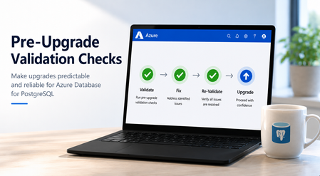
At Microsoft Build 2026, we’re announcing a major wave of PostgreSQL innovation across Azure. Alongside the public preview of Azure HorizonDB, we’re delivering a broad set of enhancements for our fully managed open-source PostgreSQL service: Azure Database for PostgreSQL flexible server. These updates span performance, analytics, security, operations, resilience and migration - helping you build faster, operate with more control, secure your workloads, and modernize with confidence. Here’s a quick tour of the top flexible server announcements at Build 2026. Feature Highlights pg_ivm Extension Defender Security assessments temporal_tables Extension Cross-tenant CMK Automatic Entra token refresh libraries New Powershell module: Az.PostgreSQLFlexibleServer More control over planned maintenance Pre-Upgrade validation checks New Built-in Grafana dashboards Chaos Studio supports Azure Database for PostgreSQL AI-assisted Oracle to PostgreSQL migration Migration Service for Azure Database for PostgreSQL improvements (EDB, AlloyDB) Performance, Scale & Analytics pg_ivm Extension Generally Available Materialized views are a useful way to optimize performance for queries that run regularly, but if underlying data becomes stale the result set needs to be recomputed. With the pg_ivm extension you can automatically maintain materialized views as the underlying data changes. This is particularly valuable for large datasets with small incremental changes that need real-time freshness, like dashboards, catalog analytics and SaaS usage reporting. We are pleased to announce the pg_ivm extension is now generally available in Azure Database for PostgreSQL. Learn more: pg_ivm. Security, Auditing & Identity Defender security assessments Preview Microsoft Defender Security Assessments for Azure Database for PostgreSQL enables continuous evaluation of your database security posture, helping identify vulnerabilities and misconfigurations across server and database configurations. Previously limited to reactive threat detection, in the latest preview release, Defender now provides proactive, risk-based insights through assessments tailored to PostgreSQL-specific best practices, delivering more relevant and actionable guidance. This helps you strengthen your security baseline, prioritize remediation, and align with best practices and compliance requirements. Learn more: https://aka.ms/Defender-Assessments-for-PG-Preview temporal_tables Extension Generally Available We’ve had many customer requests to support the temporal_tables extension, which provides built-in support for tracking and querying historical changes to data over time. Temporal tables are now generally available in Azure Database for PostgreSQL. With this extension enabled you can easily perform time-based queries, audit data changes, and maintain historical records without building custom tracking logic, simplifying application development and compliance scenarios. Learn more: temporal_tables Cross-tenant CMK Preview Azure Database for PostgreSQL now supports cross-tenant customer-managed keys (CMK) in public preview, allowing you to encrypt your data at rest using an Azure Key Vault key that resides in a separate Microsoft Entra tenant from the database service. This feature is designed for SaaS providers and enterprises that need to maintain strict separation of duties and ownership of encryption keys, enabling you to retain full control over key lifecycle management while PostgreSQL runs in a service provider’s tenant. Learn more: Data encryption at rest in Azure Database for PostgreSQL Automatic Entra token refresh libraries Preview We’re making it easier to use Entra ID authentication with Azure Database for PostgreSQL throughout the application stack by introducing new token refresh libraries for .NET, JavaScript, and Python. With Entra ID, access tokens are short-lived which can make managing their lifecycle complex in real-world applications. Developers need to be aware of token refresh and build additional handling around token expiration, connection retry, and session continuity. These new libraries remove that friction. By handling Entra token refresh seamlessly in the background, they allow applications to stay connected without interruption and with no custom logic required. The result is a simpler development experience and more resilient applications, especially for long-running or connection-heavy workloads. Across languages, the libraries provide a consistent and streamlined way to adopt secure, passwordless authentication, helping teams focus more on building their applications and less on managing authentication. Learn more: .NET, JavaScript, and Python. Operations, Maintenance & Monitoring New Powershell module: Az.PostgreSQLFlexibleServer Generally Available We’re excited to introduce the newly renamed Az.PostgreSQLFlexibleServer PowerShell module, delivering a streamlined experience for managing Azure Database for PostgreSQL with PowerShell. Building on the capabilities of the previous Az.PostgreSql module, the updated module aligns with the new features in the 2026-01-01 preview REST API. This module brings support for PostgreSQL 18, elastic clusters for scalable workloads and a range of enhancements designed to simplify management and improve performance. Whether you're provisioning new deployments or managing complex environments, this module ensures you can take full advantage of the latest platform capabilities directly from PowerShell. To learn more, visit our official documentation on PowerShell: Az.PostgreSql Module | Microsoft Learn More control over planned maintenance Generally Available We’ve seen many requests to provide more control when a maintenance update is applied to Azure Database for PostgreSQL. Sometimes when a critical workload is running you want to apply the maintenance when you’re ready. Announcing general availability this week, we’re building on the existing System and Custom maintenance window options and adding new self-service maintenance capabilities to the Azure portal. You can now reschedule upcoming maintenance updates for up to two weeks and apply maintenance on demand at a time that suits you. You can also view scheduled maintenance and review your server’s maintenance history after updates are complete. These options help you better align maintenance with your business schedules, reduce disruption during critical workload periods, and minimize the need for support-driven deferral requests. CLI and API support are coming soon. Learn more: https://aka.ms/azure-postgres-reschedule-maintenance Pre-Upgrade validation checks Preview Major version upgrades are critical for staying current with PostgreSQL features, security updates, and performance improvements, but you often discover blockers only after starting the upgrade workflow. Pre-Upgrade Validation Checks lets you validate upgrade readiness before initiating the actual upgrade by running Azure-specific upgrade checks and PostgreSQL pg_upgrade --check validations independently. The shift is simple: you can identify and fix upgrade blockers before the upgrade window begins. The feature surfaces actionable issues across configurations, extensions, dependencies, replication slots, event triggers, and other upgrade-sensitive objects. You can fix blockers, re-run validation until all checks pass, and proceed with the upgrade with greater predictability. Learn more: https://aka.ms/pg-flex-upgrade-checks New Built-in Grafana dashboards Generally Available Grafana dashboards are now built directly into the Azure portal for Azure Database for PostgreSQL - no setup, no extra cost, and no separate service to manage. You can open your PostgreSQL resource in the portal and immediately access prebuilt dashboards for key health and performance signals such as CPU, memory, storage, IOPS, connections, transactions, and availability. The key value is metrics + logs in one place. You can quickly correlate performance spikes with PostgreSQL logs, understand what changed, and troubleshoot faster using the familiar Grafana experience. Dashboards can also be customized, saved to your subscription, and shared across teams for ongoing operations. Learn more: https://aka.ms/azure-postgres-dashboards-grafana Resilience & Business Continuity Chaos Studio supports Azure Database for PostgreSQL Preview No matter how much you prepare, you only really know how good your database disaster recovery plan is when something breaks. With Chaos Studio support for Azure Database for PostgreSQL, you can simulate zone-down scenarios on PostgreSQL HA-enabled instances and validate the resilience of your mission-critical workloads. With Chaos Studio integration, you can proactively test failover behavior and gain confidence in how your applications respond to real-world zonal failures. This feature is currently available through a gated private preview. To get started, submit your subscription details using the form. Once reviewed, our team will enable the feature for your subscription, with guidance to help you begin testing. Getting started is simple: Create a Chaos Studio workspace via the Chaos Studio portal and configure your subscription, resource group, and region. Define the scope and assign the required managed identity and permissions. Review and verify your workspace setup. Browse available scenarios and select the PostgreSQL zone-down scenario. Configure the test (name, duration), then run it from My Library to begin validating failover behavior. With just a few steps, you’ll be able to simulate real-world failure conditions and gain confidence in your application’s resilience. To get started, please submit your details using this link: Private Preview Support for Chaos Studio Migration & Modernization AI-assisted Oracle to PostgreSQL migration Generally Available AI-assisted migration tooling has dramatically lowered the bar for moving between different databases and is changing the way people look at the return on investment for migration. The VS Code PostgreSQL extension comes with AI-Assisted migration tooling which converts Oracle schema and application code to Azure Database for PostgreSQL. This tooling uses GitHub Copilot, Microsoft Foundry, and custom Language Model tools to convert Oracle schema, database code and client applications into the PostgreSQL equivalents, and validates every change against a running flexible server instance. Learn more: Schema conversion, App conversion. Migration Service for Azure Database for PostgreSQL improvements (EDB, AlloyDB) Generally Available We’ve added AlloyDB and EDB Extended Server as new sources for migrating to PostgreSQL in the Azure Database for PostgreSQL Migration Service, with support for both online and offline migration support. Learn more: Migrate from AlloyDB, Migrate from EDB. Looking ahead That wraps up the Build 2026 announcements for Azure Database for PostgreSQL flexible server. There are also many great PostgreSQL technical sessions at Build this week, covering cloud-native app & AI development and migration. To find out more, here's a link to the Build session catalog for PostgreSQL sessions: https://aka.ms/Postgres-on-Azure_Build-2026. We'll continue to build out our roadmap over the coming months to deliver on your asks to improve the performance, security and stability of your PostgreSQL workloads. Check the Microsoft Blog for PostgreSQL for a regular monthly recap where we share the latest enhancements and product updates.1.6KViews2likes0CommentsLog Insights in Minutes: A Simpler pgBadger Workflow
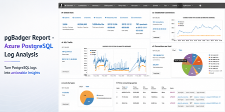
Sometimes the fastest way to understand a PostgreSQL workload is not another dashboard. It is a good log report. pgBadger is a PostgreSQL log analysis tool that turns raw PostgreSQL logs into an interactive HTML report. It helps summarize query activity, connection patterns, errors, temporary files, lock waits, autovacuum activity, and more. Earlier guidance for generating pgBadger reports from Azure Database for PostgreSQL Flexible Server focused on exporting logs through Diagnostic Settings, storing them in a storage account, and then using tools such as BlobFuse and jq to extract PostgreSQL log lines from JSON files. That workflow is still useful when customers centralize logs across multiple servers. However, if you are already using the Server logs feature in Azure Database for PostgreSQL Flexible Server, there is a much simpler path. In this post: You’ll learn how to generate a pgBadger HTML report from Azure Database for PostgreSQL Flexible Server by downloading native PostgreSQL .log files directly from the Azure portal. No storage account, BlobFuse mount, or JSON extraction required. Fast path Configure log_line_prefix . Enable Server logs for download. Download the PostgreSQL .log files. Run pgBadger with the matching prefix. Open pgbadger-report.html . Why use this workflow? With Server logs, you can download native PostgreSQL .log files directly from the Azure portal and run pgBadger locally. Older path Simpler path in this blog Diagnostic Settings → Storage account → BlobFuse → JSON extraction → pgBadger Server logs → Download .log files → pgBadger Area Older Diagnostic Settings workflow Server logs workflow Export path Diagnostic Settings to storage account Download .log files directly from the portal Format JSON payloads need extraction Native PostgreSQL .log files Extra tooling BlobFuse and jq JSON parsing None Best suited for Centralized or multi-server logging Quick per-server analysis Outcome Flexible, but more setup Faster path to pgBadger Recommended: Use the Server logs workflow when you want a fast, low-friction way to generate a pgBadger report from one Azure Database for PostgreSQL Flexible Server. When should you use this workflow? Use this workflow when... Use Diagnostic Settings when... You need a quick report for one Flexible Server. You centralize logs from many servers. You want to run pgBadger locally. You need long-term retention or workspace-level querying. You want to avoid JSON extraction. You already have automated log export pipelines. Before you start A machine where you can install or run pgBadger. A working Perl runtime. Git Bash on Windows, so the multi-line shell commands work as shown. Portal access to your Azure Database for PostgreSQL Flexible Server. Permission to update server parameters and enable Server logs. Important: pgBadger can only analyze what PostgreSQL logs capture. To populate query timing and slow-query sections in the report, enable log_min_duration_statement before collecting logs. Logs collected before that change will not include duration data. Workflow overview Task Type Rough effort Install or prepare pgBadger One-time setup per analysis machine 5–10 minutes Configure log_line_prefix One-time setup per server 2–3 minutes Enable Server logs One-time setup per server 2–3 minutes Download logs and run pgBadger Repeatable 2–5 minutes Install or prepare pgBadger on the machine where you will analyze logs. Configure log_line_prefix so pgBadger can parse each log line. Enable Server logs, so PostgreSQL logs are available for download. Download the logs and run pgBadger locally. 💡Pro tip: Start with a narrow log window first. Use one or two hourly log files, confirm the report looks right, and then expand the analysis window if needed. Step 1: Install pgBadger Before generating a report, you need pgBadger available on the machine where you plan to analyze the downloaded PostgreSQL log files. Run this on a Linux VM, WSL, or another Linux-based environment where you can install packages. Note: Azure Cloud Shell may work for quick testing, but package installation and build-tool availability can vary by session. For repeatable analysis, use a Linux VM, WSL, or another environment you control. Copy and run sudo apt-get update && sudo apt-get install -y git perl make gcc && \ git clone https://github.com/darold/pgbadger.git && \ cd pgbadger && \ perl Makefile.PL && \ make && \ sudo make install && \ pgbadger -V What good looks like: The install command completes successfully and pgbadger -V returns the installed pgBadger version. Step 2: Configure log_line_prefix This is a one-time server configuration step. The log_line_prefix parameter controls the beginning of each PostgreSQL log line. pgBadger uses this prefix to extract useful fields such as timestamp, user, database, and process ID. In the Azure portal, open your Flexible Server and go to Server parameters. Search for: Parameter log_line_prefix Set this value %m user=%u db=%d pid=%p: Then select Save. In Server parameters, confirm that the custom value is saved for log_line_prefix . Figure 1: Set log_line_prefix so pgBadger can correctly parse timestamp, user, database, and process ID from each log line. Prefix tokens Token Meaning %m Timestamp with milliseconds %u Username %d Database name %p Process ID After this change, log lines should look like this: Example log line 2026-06-22 19:00:00.070 UTC user=pgadmin db=highcpu pid=3805603: LOG: statement: SELECT 1 FROM pg_extension WHERE extname='pg_stat_statements' The matching pgBadger prefix for this log format is: Matching pgBadger prefix %m user=%u db=%d pid=%p: You will use this same value later in the pgBadger command. What good looks like: The server parameter is saved, and new PostgreSQL log lines begin with timestamp, user, database, and process ID fields that match the pgBadger prefix. Step 3: Enable Server logs for download This is also a one-time setup step. In the Azure portal, open your Flexible Server and go to Server logs. Enable: Portal setting Capture logs for download Set the retention period based on how long you want logs to remain available for download. For example, a 7-day retention period keeps logs available for download for 7 days. In Server logs, enable Capture logs for download and choose the retention window. Figure 2: Enable Capture logs for download and set a retention period long enough to cover the analysis window you want to inspect. What good looks like: After Server logs are enabled, hourly PostgreSQL log files appear in the Server logs blade and can be downloaded from the Azure portal. Once enabled, hourly log files appear in the Server logs blade. The files are named by date and hour, for example: Example log files postgresql_2026_06_22_19_00_00.log postgresql_2026_06_22_20_00_00.log Step 4: Download and organize the logs locally From the Server logs page, select the .log files for the time window you want to analyze and download them. For example, to analyze activity between 19:00 and 21:00 UTC, download: Example files to download postgresql_2026_06_22_19_00_00.log postgresql_2026_06_22_20_00_00.log On your local machine, create a folder for that analysis window. A simple convention is to use the Mon-DD format. Folder name Jun-22 Place the downloaded .log files inside that folder. Your local folder structure should look like this: Folder structure pgbadger-13.1/ pgbadger Jun-22/ postgresql_2026_06_22_19_00_00.log postgresql_2026_06_22_20_00_00.log Step 5: Generate the pgBadger report Open Git Bash from the folder where pgBadger is located. For example, if pgBadger is inside the pgbadger-13.1 folder, open Git Bash from that folder. # Action Command 1 Set the folder FOLDER=Jun-22 2 Confirm files ls -lh ./$FOLDER 3 Run pgBadger Use the full command below. Copy and run FOLDER=Jun-22 ls -lh ./$FOLDER perl -X ./pgbadger -f stderr \ --prefix '%m user=%u db=%d pid=%p:' \ ./$FOLDER/*.log \ -o ./$FOLDER/pgbadger-report.html Command breakdown Part of command Purpose perl -X ./pgbadger Runs pgBadger and suppresses non-critical Perl warnings. -f stderr Parses PostgreSQL stderr log files. --prefix '%m user=%u db=%d pid=%p:' Matches the log_line_prefix set on the server. ./$FOLDER/*.log Analyzes every .log file in the selected folder. -o ./$FOLDER/pgbadger-report.html Writes the HTML report into the same folder. When the command completes successfully, you should see output like this: Expected output Parsed 12134249 bytes of 12134249 (100.00%), queries: 26684, events: 83 LOG: Ok, generating html report... What good looks like: pgBadger finishes parsing the logs and creates pgbadger-report.html in the selected folder. Step 6: Open the report Open the generated report: Copy and run start ./$FOLDER/pgbadger-report.html The report opens in your default browser. The final report is created here: Generated report path Jun-22/pgbadger-report.html What the report can show The pgBadger report gives you a quick view into the workload shape for the selected log window. For example, in a sample run across two hourly log files, pgBadger summarized: Total number of queries. Number of unique normalized queries. Query traffic over time. Events such as errors and fatal messages. Session and connection patterns. Once the report opens, start with Global Stats to confirm the time range, total queries, normalized queries, and query peak. Figure 3: Start with Global Stats to validate the selected time range, total query count, normalized query count, and query peak. Query volume and normalized queries Many raw queries can often reduce to a smaller number of normalized query patterns. This helps identify whether the workload is spread across many different query shapes or dominated by a smaller set of repeated statements. Example: In this sample run, 26,684 queries reduced to 59 normalized query shapes. That suggests the workload is mostly a small set of repeated statements, which can help focus tuning effort. Traffic patterns The SQL Traffic section helps identify spikes, quiet periods, and workload changes over time. Figure 4: Use SQL Traffic to identify query spikes, quiet periods, and workload changes during the selected log window. Figure 5: Review the query breakdown to compare read vs. write volume and query-type distribution for the selected Server logs window. For example, if the report shows a steady baseline followed by a sharp spike, that spike can be correlated with application activity, batch jobs, synthetic tests, or operational events during the same time window. Query duration If query duration shows 0 ms or the slow query sections are empty, it usually means duration logging was not enabled when the logs were collected. In that case, pgBadger can still show query counts and events, but it cannot calculate the slowest queries, total execution time, average duration, or maximum duration. To unlock those timing sections, enable log_min_duration_statement , collect fresh logs, and rerun pgBadger. What pgBadger cannot infer from missing logs pgBadger reports are only as complete as the log data you provide. If PostgreSQL did not log duration, lock waits, temporary files, or autovacuum activity during the selected time window, pgBadger cannot reconstruct those details later. To analyze... Enable before collecting logs Slow queries log_min_duration_statement Lock waits log_lock_waits Temporary files log_temp_files Autovacuum activity log_autovacuum_min_duration Repeatable copy/paste block Reusable command block Change only FOLDER for each new analysis window. Copy and run FOLDER=Jun-22 ls -lh ./$FOLDER perl -X ./pgbadger -f stderr \ --prefix '%m user=%u db=%d pid=%p:' \ ./$FOLDER/*.log \ -o ./$FOLDER/pgbadger-report.html start ./$FOLDER/pgbadger-report.html For another date, change only this line: Update this value FOLDER=Jun-22 Examples: Example folder values FOLDER=Jun-23 FOLDER=Jul-01 FOLDER=Aug-15 Optional: Improve report quality pgBadger can only analyze the information captured in PostgreSQL logs. The default logs may be enough for query frequency, connection activity, and errors. For deeper performance troubleshooting, consider enabling additional logging parameters based on your scenario. Scenario Parameter Suggested value Notes Slow query analysis log_min_duration_statement 1000 Logs statements slower than 1 second. Short controlled test log_min_duration_statement 0 Logs every statement. Use carefully. Lock troubleshooting log_lock_waits on Helps identify lock waits. Temporary file analysis log_temp_files 0 Logs all temporary files. Autovacuum visibility log_autovacuum_min_duration 0 Useful during focused analysis. Useful parameters include: Recommended logging parameters log_lock_waits = on log_temp_files = 0 log_autovacuum_min_duration = 0 To capture query durations, configure: Duration logging log_min_duration_statement = 1000 This logs statements that run longer than 1000 milliseconds. For short test runs, you can temporarily use: Short test run only log_min_duration_statement = 0 Caution: Use log_min_duration_statement = 0 carefully on busy production servers. It logs every statement and can generate a large volume of logs. Duration matters: If duration logging is not enabled, pgBadger can still show query counts and events, but slowest-query, total duration, average duration, and maximum duration sections will be limited or empty. Common mistakes and quick fixes Symptom Likely cause Fix Report is empty Prefix mismatch Match --prefix with log_line_prefix . No duration data Duration logging was not enabled Set log_min_duration_statement before collecting logs. No files visible Server logs disabled or retention expired Enable capture and check retention. pgBadger command fails pgBadger is not in the current folder or path Run pgbadger -V to confirm installation. Common troubleshooting FAQs 1. Report is created but empty This usually means the pgBadger prefix did not match the actual log format. Check the first few lines: Copy and run head -5 ./$FOLDER/*.log Make sure the pgBadger --prefix matches the server’s log_line_prefix . 2. Report shows queries but no duration PostgreSQL logged statements but did not log durations. Enable one of the following, collect fresh logs, and rerun pgBadger: Parameter options log_min_duration_statement = 1000 # or temporarily for testing log_min_duration_statement = 0 3. No .log files are visible Confirm that Server logs are enabled: Portal setting Capture logs for download Also check the retention period. If the retention period has expired, older logs may no longer be available for download. 4. pgBadger command fails Confirm that pgBadger is available in the current folder or installed in your path. Copy and run pgbadger -V If you are running pgBadger from the local folder, use: Copy and run perl -X ./pgbadger Summary For customers already using Azure Database for PostgreSQL Flexible Server logs, the pgBadger workflow is straightforward: Install pgBadger. Configure log_line_prefix . Enable Server logs for download. Download the .log files. Place them in a local date-based folder. Run pgBadger with the matching prefix. Open pgbadger-report.html . Bottom line: Server logs give you the shortest path from Azure Database for PostgreSQL Flexible Server logs to a pgBadger report. Download the native .log files, run pgBadger with the matching prefix, and open the generated HTML report. References pgBadger - source and documentation GitHub pgBadger - project site Azure - Download server logs from the portal Flexible Server Azure - Logging concepts Flexible Server Azure - Configure server parameters via the portal PostgreSQL - log_line_prefix and logging parameters673Views2likes0CommentsMultitude builds resilient banking platform with PostgreSQL and MySQL on Azure
Expanding into new markets is usually a sign that things are going well. For digital banking platforms, however, growth brings a different kind of challenge - more customers, more data, and stricter expectations around availability, security, and regulatory compliance. At Multitude, we operate across 17 countries and deliver digital banking, credit services, payment processing, and regulatory reporting through a platform composed of more than 400 microservices. Each service encapsulates a defined business capability, including onboarding, risk assessment, collections, and compliance workflows. Historically, our services relied on on-premises PostgreSQL and MySQL environments deployed within our own data centers, where capacity scaled vertically on shared compute and storage resources. This model created contention between unrelated workloads and limited their ability to scale independently. Expanding capacity required adding or upgrading physical hardware, which involved demand forecasting, procurement, delivery coordination, and installation within the data center. Over time, continued growth amplified these architectural constraints. The database engines themselves remained reliable, but the surrounding infrastructure limited elasticity and domain-level isolation. As a result, sustained growth began to expose structural limits in the underlying infrastructure. "In a regulated financial environment, those constraints carried broader implications. Frameworks such as DORA and GDPR require predictable availability, controlled recovery procedures, and governed access to sensitive data. As workload demands increased, sustaining both growth and compliance required structural changes at the database layer. We decided that redesigning our data architecture was necessary to improve workload isolation, scalability, and governance alignment. Rearchitecting data boundaries with Azure Databases We initiated our architectural redesign by migrating database workloads to Microsoft Azure and standardizing on Azure Database for PostgreSQL and Azure Database for MySQL for core application services. Central to this redesign was the adoption of bounded contexts. Each bounded context represents a logical business domain and encapsulates the services and schemas required to support that capability. Each domain is owned and managed by a single team, aligning technical boundaries with team responsibility and accountability. Rather than maintaining a small number of large, shared database instances, we provisioned dedicated database instances aligned to defined business domains, establishing domain-level isolation at the database layer. Today, approximately 35 database instances support more than 400 microservices across the platform. Each instance may host multiple schemas serving related services within the same domain, while cross-domain database dependencies are intentionally avoided. This structure limits the blast radius of configuration changes or workload spikes and allows scaling adjustments to be applied within clearly defined domain boundaries. While the bounded context model was a strategic architectural decision, leveraging managed database services helped us implement it by drastically reducing the operational overhead of provisioning, scaling, and maintaining independent instances across domains. Azure Database for PostgreSQL and Azure Database for MySQL provide the managed capabilities required to sustain this model. Instances are provisioned according to the performance and storage requirements of each domain and can be adjusted as workload characteristics evolve. Compute and storage resources are scaled at the instance level, allowing capacity changes to be applied to a specific bounded context without affecting unrelated domains. Altogether, these architectural decisions balance domain-level isolation with operational manageability. A database-per-microservice pattern would significantly increase provisioning, monitoring, and lifecycle overhead without materially improving data ownership boundaries. By grouping related services within bounded contexts, we maintain clear domain alignment while keeping the number of database instances practical to operate. As a result, data boundaries, scaling behavior, and operational controls remain consistent with business domain structures across the platform. Operationalizing high availability and backup strategy To support availability, we deploy Azure Database for PostgreSQL and Azure Database for MySQL with zone-redundant high availability, placing primary and standby replicas in separate availability zones within the same Azure region. Replication preserves transactional consistency, and zone separation reduces exposure to localized infrastructure failures. We periodically exercise failover procedures as part of operational validation to confirm recovery behavior under defined conditions. Availability controls are complemented by a layered backup strategy. Azure Database for PostgreSQL and Azure Database for MySQL provide automated backups with a retention window of up to 35 days and point-in-time restore capabilities. These features allow us to restore a database to a specific timestamp within the retention window, supporting recovery from application-level errors or unintended data modifications without custom snapshot orchestration. Together, operational backups and governed archival retention address both short-term recovery and long-term compliance obligations. Restore operations require documented justification and follow established approval workflows, ensuring that recovery actions remain controlled, traceable, and auditable. We also enforce consistency through lifecycle management. Azure’s managed service model standardizes engine patching and version updates across environments, reducing configuration drift and minimizing manual coordination. By operating within the managed service boundary, the database team can focus on workload analysis, performance tuning, and capacity planning. For migration and synchronization scenarios, we use Azure Data Migration Service to orchestrate controlled cutovers between database environments. Engineers validate configuration and readiness before initiating synchronization, after which Azure-managed replication then maintains data alignment until final switchover. Provisioning decisions and structural modifications remain subject to internal governance approvals to preserve change control and oversight. By combining zone-redundant availability, structured recovery workflows, governed retention policies, and standardized lifecycle management, we operate a database layer engineered for resilience, auditability, and regulatory alignment at scale. Compliance as an architectural property For us, governance is embedded directly into how the platform operates, beginning at the identity layer. Access to Azure Database for PostgreSQL and Azure Database for MySQL integrates with Microsoft Entra ID, aligning database authentication with centrally managed corporate identities. Role-based access control is enforced through enterprise identity policies, providing centralized visibility into access assignments and authentication events across environments. These controls extend into production access management. Privileged access is approval-based and time-bound, and administrative roles are not permanently assigned. Access requests follow defined workflows, and all privileged actions are logged for review under established oversight procedures, ensuring traceability of operational interventions. Database isolation reinforces these identity controls. By aligning database instances with bounded contexts, each business domain maintains a discrete data boundary at the database layer. This structure limits lateral access across domains and confines sensitive data to clearly defined ownership scopes, simplifying monitoring and audit review. In a regulated financial environment, these architectural controls also support compliance requirements under frameworks such as DORA and GDPR. By embedding identity integration, domain isolation, and lifecycle controls directly into the platform architecture, governance becomes an operational property of the system rather than a separate procedural layer. The simplicity of this architecture is a strong driver for both auditability and security of the whole platform. Measurable impact across engineering teams and business outcomes Beyond improved stability, our ability to respond to growth has changed significantly since moving to Azure. In the past, expanding database capacity meant procuring hardware and planning installation in the data center. Now, capacity adjustments happen directly within Azure and can be applied to individual databases instances, allowing us to scale in near real time as workload demands change. Maintenance effort has also decreased. Managed patching, version alignment, and automated backups have reduced the need for manual coordination and reactive capacity management. Infrastructure-level tasks that once required continuous oversight are now handled within the managed service boundary. Our DBAs are now focused on improving performance and stability. We spend far less time maintaining the basics. Resilience by design The structural changes behind these results reflect a deliberate long-term strategy. Our database architecture now aligns with the operating model we expect to sustain over the next five years and beyond. Bounded contexts define discrete data domains, while Azure Database for PostgreSQL and Azure Database for MySQL provide managed high availability, scaling controls, and standardized lifecycle management across those domains. Identity integration and governed recovery procedures operate consistently across environments. With this architecture in place, Multitude scales responsibly in regulated markets while maintaining strict governance and availability standards. Expanding into new markets still means more customers and more data - but now our platform is designed to handle that success.640Views3likes0CommentsJune 2026 Recap: Azure Database for PostgreSQL
POSETTE 2026 We hosted POSETTE: An Event for Postgres 2026 in June! This year marked our 5th annual event featuring 50 speakers and a total of 44 talks. PostgreSQL developers, contributors, and community members came together to share insights on topics covering everything from AI-powered applications to deep dives into PostgreSQL internals. If you missed it, you can catch up by watching the POSETTE livestream sessions. If this conference sounds interesting to you and want to be part of it next year, don’t forget to subscribe to POSETTE news. Features 💡 Chaos Studio Workspaces for Azure Database for PostgreSQL Flexible Server – Public Preview Chaos Studio Workspaces now support Azure Database for PostgreSQL Flexible Server in Public Preview. You point a Workspace at a subscription or resource group, and Chaos Studio discovers your Flexible Server instances and recommends a PostgreSQL zone-down failover Scenario. The Scenario requires a Flexible Server with High Availability enabled. Running the Scenario simulates an availability-zone outage, drives an HA failover, and produces a Scenario report of exactly what happened. Read more here: https://aka.ms/ChaosStudioPostgreSQL Try it today: https://aka.ms/chaos-portal Microsoft Defender Security Assessment for Azure Database for PostgreSQL - General Availability Microsoft Defender security posture assessments for Azure Database for PostgreSQL Flexible Server are now generally available. Built-in assessments continuously evaluate PostgreSQL configurations against PostgreSQL-specific security best practices, helping identify vulnerabilities and misconfigurations with actionable remediation guidance. Customers can use these assessments to strengthen their security baseline, prioritize remediation efforts, and support compliance requirements. Assessments are automatically available for servers already protected by Microsoft Defender for Cloud Security Posture Management (CSPM), with no additional setup required. An initial set of assessments is available today, with additional coverage planned for future releases to help strengthen the security posture of PostgreSQL workloads. Read more here: Microsoft Defender for Cloud - Azure Database for PostgreSQL | Microsoft Learn DROP CAST Support added Custom casts can be useful when applications need to convert between data types in a way that matches their business logic or migration requirements. Previously, while you could create custom casts, it wasn’t possible to drop them once they were no longer needed. With this update, you can now use the PostgreSQL DROP CAST command to clean up unused or obsolete casts, making it easier to manage schema customizations over time. Example: CREATE CAST (bigint AS text) WITH INOUT; … DROP CAST IF EXISTS (bigint AS text); Latest PostgreSQL minor versions: 18.4, 17.10, 16.14, 15.18, 14.23 Azure Database for PostgreSQL now supports the latest PostgreSQL minor versions: 18.4, 17.10, 16.14, 15.18, and 14.23. These updates are applied automatically during planned maintenance windows, helping keep your databases current with the latest PostgreSQL community fixes and reliability improvements, with no manual action required. This release includes fixes across query correctness, planner behavior, replication, backup and restore tooling, logical replication, foreign data wrapper behavior, and timezone data, improving overall stability and correctness of database operations. For details about the minor release, see the PostgreSQL announcement. Azure PostgreSQL Learning Bytes 🎓 Generate a pgBadger report from Server Logs Need a quick workload readout from PostgreSQL logs? Use pgBadger with Azure PostgreSQL Server Logs. Fast path: Server logs → Download '.log' files → Generate pgBadger report Before collecting logs, set log_line_prefix in Server parameters: %m user=%u db=%d pid=%p: Then enable Server logs > Capture logs for download, download the .log files for the time window you want to analyze, place them in a local folder, and run: FOLDER=<logs-folder-name> pgbadger -f stderr \ --prefix '%m user=%u db=%d pid=%p:' \ ./$FOLDER/*.log \ -o ./$FOLDER/pgbadger-report.html Open the generated report: start ./$FOLDER/pgbadger-report.html This gives you a quick HTML report for query activity, connection patterns, events, lock waits, and workload spikes - without setting up a storage account, BlobFuse mount, or JSON extraction pipeline. 💡Tip: Start with one or two hourly log files first. Confirm the report looks right, then expand the log analysis window. Learn more: Log Insights in Minutes: A Simpler pgBadger Workflow292Views1like0CommentsSELECT * FROM build2026_sessions WHERE postgres = true;
Microsoft Build 2026 is around the corner, and this year it’s shaping up to be a big one for PostgreSQL experts and enthusiasts. If you’re a developer working with Postgres, or just love exploring new database technology, there's plenty to get excited about. Microsoft’s new cloud-first evolution of PostgreSQL, Azure HorizonDB, alongside sessions featuring Azure Database for PostgreSQL, will highlight how Postgres is powering the next wave of AI-driven applications. A new horizon in Postgres Build 2026 arrives at a time when the role of databases in modern apps is evolving rapidly. From enabling AI model integration to scaling seamlessly across the cloud, PostgreSQL developers today are dealing with more complex demands than ever. That’s why Azure HorizonDB – Microsoft’s new cloud-native PostgreSQL service – is generating so much buzz ahead of Build. What is Azure HorizonDB? In short, it’s a reimagined version of PostgreSQL designed for cloud-scale performance and AI-era workloads. Azure HorizonDB, introduces a distributed architecture that decouples compute and storage, delivering sub-millisecond latencies and three times the throughput of self-managed Postgres at massive scale. It aims to preserve Postgres’s beloved features and SQL ecosystem while adding next-generation capabilities: built-in vector indexing for high-speed AI/ML retrieval, the ability to run AI models and vector operations directly in the database, and multi-zone replication for resilience. For Postgres developers, this means less time stitching together external data stores or machine learning services – and more time building powerful apps on a unified platform that’s both familiar and built for the future. The bottom line: Microsoft Build 2026 is an ideal opportunity for developers to see Azure HorizonDB in action, learn best practices for modern PostgreSQL architectures, and understand how to leverage Postgres in new scenarios like generative AI and multi-agent applications. Read on for a rundown of sessions covering these topics, complete with what you’ll learn from each one. Top sessions for PostgreSQL databases on Azure Below are key sessions tailored for PostgreSQL users and those interested in Azure HorizonDB, with session types and highlights of what you’ll gain by attending. 🎤 Breakout: From Rows to Reasoning: Designing Databases for AI Apps and Agents (BRK223, 45 min, in-person and digital options) Discover how to architect databases that can power tomorrow’s intelligent applications. This technical breakout will show how AI-ready databases can move beyond plain transactions. You’ll see live demos of integrating transactional, analytical, and vector data in one unified platform, with Azure’s new database capabilities, including Azure HorizonDB. Learn how to simplify your stack by eliminating separate analytics engines or vector stores. The session will highlight patterns that reduce data movement and latency so your apps can efficiently reason over live data with minimal complexity. 🧪 Hands-on lab: Create Advanced Postgres-Powered Agentic Apps with Azure HorizonDB (LAB511, 75 min, in person and digital options) Roll up your sleeves and get hands-on building a real multi-agent AI application with Postgres. In this advanced lab, you’ll create a production-ready AI agent powered by Azure HorizonDB as an all-in-one data, search, and intelligence layer. Experiment with retrieval-augmented generation (RAG) by combining semantic vector search (DiskANN) with traditional SQL queries right inside the database. Implement hybrid search and agent workflows without resorting to external vector databases or glue code – thanks to HorizonDB’s built-in vector indexing and in-database AI model capabilities. This lab is perfect for developers who want to experience how HorizonDB can simplify your stack and boost performance for AI-driven apps. Multiple hands-on labs are offered to suite your schedule. 💻 Demo: Simplify App Dev with Cloud-Native PostgreSQL in Azure HorizonDB (DEM364, 25 min, in-person and digital options) See how to cut your development time and complexity with built-in AI and search features in Postgres. This fast-paced demo shows how Azure HorizonDB helps eliminate the need for separate search engines and AI services by pulling those capabilities straight into PostgreSQL. Expect to learn how you can run hybrid vector + keyword queries using SQL, integrate AI models directly from within the database, and apply full-text search (BM25) and semantic ranking to get smarter results. If you’re eager to deliver intelligent apps faster, with fewer moving parts, this session will show how HorizonDB simplifies your architecture without sacrificing performance. ⚡Lightning Talk: Cloud-Native PostgreSQL, Rebuilt for Scale: Azure HorizonDB (LTG413, 15 min, in-person only) Get a rapid-fire introduction to the architecture behind HorizonDB’s eye-popping performance. This short talk dives into how HorizonDB re-architects core PostgreSQL to deliver effortless scale out and blazing speed. Learn how decoupled compute and storage, predictive caching, and multi-region replication combine to achieve sub-millisecond query latencies and 3× higher throughput than standard Postgres. If you care about performance tuning and high-scale database design, don’t miss this quick primer on the tech under HorizonDB’s hood. 👥 Interactive Table Talk: Scaling PostgreSQL for AI Apps: Patterns and Tradeoffs (TT622, 45 min, in-person only) Bring your questions and ideas to this collaborative discussion. In this open round-table session with community and Microsoft experts, you’ll explore architecture patterns for scaling PostgreSQL to meet the demands of agent-based and AI-driven applications. Discuss real-world strategies for handling vector embeddings in Postgres, unifying relational and document data, integrating with AI models, and more. Compare the trade-offs between different scaling approaches – from monolithic to microservices, sharding strategies, and new technologies like HorizonDB – and learn where each design shines or struggles in production. Come ready to share your experiences and learn from others in the room. ▶️ On-Demand: Smarter PostgreSQL Migrations to Power Modern, Intelligent Apps (OD822, 30 min, digital only) Planning to migrate to Postgres or move your databases to Azure? Start here. This on-demand session focuses on new tools and proven strategies to migrate large-scale databases to Azure Database for PostgreSQL quickly and safely. You’ll see AI-assisted migration tools in action that minimize downtime and risk when moving terabytes of data. Just as importantly, you’ll learn how migrating to Azure unlocks advanced capabilities – from boosted performance and enhanced security to AI-ready features – helping you turn your newly migrated data into intelligent apps and services. On-demand session will be available to stream on the first day of Build. Meet the team: PostgreSQL expert meetups If you’re attending Build in person, stop by the Expert Meetup (EMU) area and head to the relational cloud databases booth. This is your chance to talk directly with the engineers and product teams behind PostgreSQL on Azure. Bring your questions about architecture decisions, scaling patterns, migrations, AI workloads, or anything else on your mind. Whether you want to sanity-check a design, dig deeper into something you saw in a session, or give direct feedback, the EMU space is designed for exactly that convo. How to get the most out of Build (and what to do next) With so much great content lined up, how do you decide where to start? It really depends on what you’re most excited about: Curious about AI and agentic apps: Start with From Rows to Reasoning, then go deeper with the Simplify App Dev with HorizonDB demo or get hands-on at the Azure HorizonDB labs to see how these ideas work in practice. Performance and scale are your focus: The short Lightning Talk on HorizonDB’s cloud-native architecture and the Table Talk on scaling Postgres will both provide unique insights and pro tips for running Postgres at massive scale. Planning a migration to PostgreSQL on Azure: Watch the Smarter PostgreSQL Migrations on-demand session to learn how to migrate large workloads with minimal downtime, and the benefits you can unlock after moving to Azure. Looking for real answers to your specific questions: Make time for the PostgreSQL Expert Meetup area to connect directly with the team. No matter which sessions you choose, Build 2026 promises to be an exciting event for the PostgreSQL developer community. Browse the session catalog, save the sessions that match your interests, and we’ll see you at Build.908Views2likes0CommentsReal-World Success Stories with PostgreSQL on Azure
Organizations rarely leap into cloud migrations or AI-powered systems overnight. They progress in deliberate stages, establishing a reliable data foundation, optimizing for performance, and then accelerating innovation. Across healthcare, financial services, and AI startups, companies are navigating this journey on Azure Database for PostgreSQL: a fully managed, enterprise-ready PostgreSQL environment with 58% lower total cost of ownership (TCO) compared to on-premises deployments. This post walks through real customer stories that span the full arc, from lift-and-shift migration to production-grade AI agent development, illustrating how Azure Database for PostgreSQL supports scalability, performance, security, and AI-readiness at every stage. Migrating with Confidence: Apollo Hospitals & August AI Apollo Hospitals operates a network of more than 74 hospitals and needed to move beyond a legacy on-premises Oracle system that had become difficult to manage and couldn't keep pace with growing data volumes. IT teams were spending their time on maintenance rather than innovation. Apollo migrated its core hospital information system backend to Azure Database for PostgreSQL. Working with partner Quadrant Technologies, the team lifted and shifted critical applications while using Azure DevOps to orchestrate CI/CD pipelines and Azure Application Insights for telemetry and observability. The results: 99.95% availability across hospital systems Database transactions executing within 5 seconds 40% reduction in deployment times via modern CI/CD pipelines Decreased operational overhead, freeing IT staff for higher-value work With a stable, scalable PostgreSQL backend in place, Apollo is now exploring real-time analytics and AI-enabled tools like Microsoft 365 Copilot to advance patient care. "We saw Azure Database for PostgreSQL as the right foundation for the future. It's open, cost-effective, and capable of supporting the hospital information system we built in-house." — Shankar Krishna A., General Manager of IT, Apollo Hospitals Apollo's experience is not unique. August AI, a healthcare-tech startup offering an AI-driven medical companion, migrated its entire stack to Azure—with Azure Database for PostgreSQL storing mission-critical patient data while meeting strict compliance requirements such as HIPAA. The result: scaling from roughly 500,000 users to 3.5 million+ users worldwide, with zero downtime during the cutover, completed in just three months. As Founder and CEO Anuruddh Mishra noted: "We receive a log of queries that are not performing optimally, and within a couple of minutes we can optimize that query with PostgreSQL on Azure and move on". Modernizing at Scale: Nasdaq Migration is often the first step. Nasdaq demonstrates what becomes possible when organizations modernize their architecture on a scalable data foundation. To improve its Nasdaq Boardvantage platform—used by corporate boards to collaborate on governance documents—Nasdaq re-architected on Azure. The team containerized services with Azure Kubernetes Service (AKS) and adopted Azure Database for PostgreSQL alongside Azure Database for MySQL as persistent data stores for governance workloads. This architecture provided the flexibility, performance, and security required for a multitenant platform handling sensitive board materials. With the data layer in place, Nasdaq integrated Microsoft Foundry and Azure OpenAI to deliver AI-powered summarization and workflow automation. The measurable outcomes: 60% reduction in reading time through AI-powered document summarization 25% decrease in administrative preparation time across board workflows Up to 97% accuracy in AI-generated summaries and meeting minutes A reusable AI framework established for future extensibility "Both Azure Database for PostgreSQL and Azure Database for MySQL gave us the right balance of performance, security, and control. The governance workloads we handle are unique, so we needed something that could meet those isolation and encryption requirements." — Scott Ellison, Vice President of Technology, Nasdaq Building Intelligent Applications: SubgenAI and OpenAI Azure Database for PostgreSQL now supports native vector search via pgvector, high-performance DiskANN indexing, semantic operators and AI model management, and integrated graph capabilities for relationship reasoning—making it a production-ready foundation for intelligent applications. SubgenAI, a European generative AI company, built its flagship platform Serenity Star on Azure Database for PostgreSQL and Microsoft Foundry to transform AI agent development from a code-heavy, fragmented process into a streamlined, no-code experience. A core technical requirement: the platform's retrieval-augmented generation (RAG) system needs efficient vector search against embedded content while maintaining enterprise-grade reliability. After evaluating several database options, SubgenAI chose Azure Database for PostgreSQL with pgvector for its accurate and scalable vector similarity search. Serenity Star customers can now: Launch AI agents in as little as 15 minutes Cut coding and development time by 50% Resolve most AI agent queries in under 60 seconds [ "With Microsoft and Azure Database for PostgreSQL we have total control and an environment that is truly dynamic and can adapt to the evolution we're looking for." — Julia Schröder Langhaeuser, VP of Product Serenity Star, SubgenAI At the extreme end of scale, OpenAI runs PostgreSQL on Azure to support production systems behind ChatGPT. As write scalability limits emerged on an initially unsharded single primary instance, OpenAI offloaded write-heavy operations to other systems and optimized read workloads using PgBouncer for connection pooling. The Azure Database for PostgreSQL team responded by developing the elastic clusters feature, enabling horizontal scaling through row-based and schema-based sharding. The team reduced connection latency from approximately 50 ms to under 5 ms, scaled reads horizontally with multiple replicas, and improved reliability by prioritizing critical requests—all achieved by a small team making systematic optimizations on open-source PostgreSQL. "After all the optimization we did, we are super happy with Postgres right now for our read-heavy workloads. It's really scalable and reliable." — Bohan Zhang, Member of the Technical Staff, OpenAI Meeting You Where You Are Beyond these stories, organizations like BMW Group (cloud-native applications at global scale), Ahold Delhaize (highly available retail applications), Mott MacDonald (an AI agent accelerating onboarding and spreading best practices across 220,000 employees), and Multitude (scaling responsibly in regulated environments) all run on Azure Database for PostgreSQL. The service offers 99.99% availability with automatic failover and SLA, independent compute and storage scaling, and intelligent performance recommendations, available across 60+ Azure regions. Developer tooling including the PostgreSQL extension for Visual Studio Code with GitHub Copilot further accelerates productivity. Whether you are planning your first migration or building production AI agents, these stories share a clear signal: Azure Database for PostgreSQL delivers a scalable, secure, AI-ready data foundation at every stage of growth. Explore full customer stories in depth in the eBook: Customer Success Stories with Azure Database for PostgreSQL.435Views2likes0Comments