onnx
23 Topics
Getting Started with the AI Dev Gallery
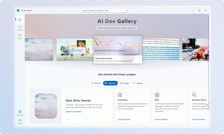
March Update: The Gallery is now available on the Microsoft Store! The AI Dev Gallery is a new open-source project designed to inspire and support developers in integrating on-device AI functionality into their Windows apps. It offers an intuitive UX for exploring and testing interactive AI samples powered by local models. Key features include: Quickly explore and download models from well-known sources on GitHub and HuggingFace. Test different models with interactive samples over 25 different scenarios, including text, image, audio, and video use cases. See all relevant code and library references for every sample. Switch between models that run on CPU and GPU depending on your device capabilities. Quickly get started with your own projects by exporting any sample to a fresh Visual Studio project that references the same model cache, preventing duplicate downloads. Part of the motivation behind the Gallery was exposing developers to the host of benefits that come with on-device AI. Some of these benefits include improved data security and privacy, increased control and parameterization, and no dependence on an internet connection or third-party cloud provider. Requirements Device Requirements Minimum OS Version: Windows 10, version 1809 (10.0; Build 17763) Architecture: x64, ARM64 Memory: At least 16 GB is recommended Disk Space: At least 20GB free space is recommended GPU: 8GB of VRAM is recommended for running samples on the GPU Using the Gallery The AI Dev Gallery has can be navigated in two ways: The Samples View The Models View Navigating Samples In this view, samples are broken up into categories (Text, Code, Image, etc.) and then into more specific samples, like in the Translate Text pictured below: On clicking a sample, you will be prompted to choose a model to download if you haven’t run this sample before: Next to the model you can see the size of the model, whether it will run on CPU or GPU, and the associated license. Pick the model that makes the most sense for your machine. You can also download new models and change the model for a sample later from the sample view. Just click the model drop down at the top of the sample: The last thing you can do from the Sample pane is view the sample code and export the project to Visual Studio. Both buttons are found in the top right corner of the sample, and the code view will look like this: Navigating Models If you would rather navigate by models instead of samples, the Gallery also provides the model view: The model view contains a similar navigation menu on the right to navigate between models based on category. Clicking on a model will allow you to see a description of the model, the versions of it that are available to download, and the samples that use the model. Clicking on a sample will take back over to the samples view where you can see the model in action. Deleting and Managing Models If you need to clear up space or see download details for the models you are using, you can head over the Settings page to manage your downloads: From here, you can easily see every model you have downloaded and how much space on your drive they are taking up. You can clear your entire cache for a fresh start or delete individual models that you are no longer using. Any deleted model can be redownload through either the models or samples view. Next Steps for the Gallery The AI Dev Gallery is still a work in progress, and we plan on adding more samples, models, APIs, and features, and we are evaluating adding support for NPUs to take the experience even further If you have feedback, noticed a bug, or any ideas for features or samples, head over to the issue board and submit an issue. We also have a discussion board for any other topics relevant to the Gallery. The Gallery is an open-source project, and we would love contribution, feedback, and ideation! Happy modeling!7.2KViews5likes3CommentsAI Toolkit for Visual Studio Code: October 2024 Update Highlights
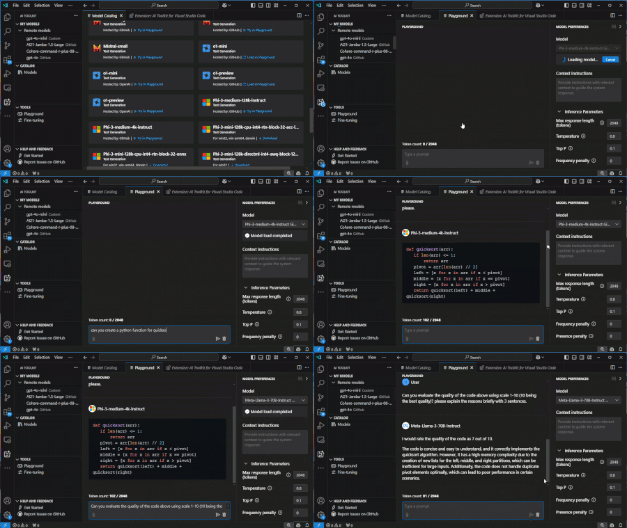
The AI Toolkit’s October 2024 update revolutionizes Visual Studio Code with game-changing features for developers, researchers, and enthusiasts. Explore multi-model integration, including GitHub Models, ONNX, and Google Gemini, alongside custom model support. Dive into multi-modal capabilities for richer AI testing and seamless multi-platform compatibility across Windows, macOS, and Linux. Tailored for productivity, the enhanced Model Catalog simplifies choosing the best tools for your projects. Try it now and share feedback to shape the future of AI in VS Code!3.2KViews4likes0CommentsOn‑Device AI with Windows AI Foundry and Foundry Local
From “waiting” to “instant”- without sending data away AI is everywhere, but speed, privacy, and reliability are critical. Users expect instant answers without compromise. On-device AI makes that possible: fast, private and available, even when the network isn’t - empowering apps to deliver seamless experiences. Imagine an intelligent assistant that works in seconds, without sending a text to the cloud. This approach brings speed and data control to the places that need it most; while still letting you tap into cloud power when it makes sense. Windows AI Foundry: A Local Home for Models Windows AI Foundry is a developer toolkit that makes it simple to run AI models directly on Windows devices. It uses ONNX Runtime under the hood and can leverage CPU, GPU (via DirectML), or NPU acceleration, without requiring you to manage those details. The principle is straightforward: Keep the model and the data on the same device. Inference becomes faster, and data stays local by default unless you explicitly choose to use the cloud. Foundry Local Foundry Local is the engine that powers this experience. Think of it as local AI runtime - fast, private, and easy to integrate into an app. Why Adopt On‑Device AI? Faster, more responsive apps: Local inference often reduces perceived latency and improves user experience. Privacy‑first by design: Keep sensitive data on the device; avoid cloud round trips unless the user opts in. Offline capability: An app can provide AI features even without a network connection. Cost control: Reduce cloud compute and data costs for common, high‑volume tasks. This approach is especially useful in regulated industries, field‑work tools, and any app where users expect quick, on‑device responses. Hybrid Pattern for Real Apps On-device AI doesn’t replace the cloud, it complements it. Here’s how: Standalone On‑Device: Quick, private actions like document summarization, local search, and offline assistants. Cloud‑Enhanced (Optional): Large-context models, up-to-date knowledge, or heavy multimodal workloads. Design an app to keep data local by default and surface cloud options transparently with user consent and clear disclosures. Windows AI Foundry supports hybrid workflows: Use Foundry Local for real-time inference. Sync with Azure AI services for model updates, telemetry, and advanced analytics. Implement fallback strategies for resource-intensive scenarios. Application Workflow Code Example using Foundry Local: 1. Only On-Device: Tries Foundry Local first, falls back to ONNX if foundry_runtime.check_foundry_available(): # Use on-device Foundry Local models try: answer = foundry_runtime.run_inference(question, context) return answer, source="Foundry Local (On-Device)" except Exception as e: logger.warning(f"Foundry failed: {e}, trying ONNX...") if onnx_model.is_loaded(): # Fallback to local BERT ONNX model try: answer = bert_model.get_answer(question, context) return answer, source="BERT ONNX (On-Device)" except Exception as e: logger.warning(f"ONNX failed: {e}") return "Error: No local AI available" 2. Hybrid approach: On-device first, cloud as last resort def get_answer(question, context): """ Priority order: 1. Foundry Local (best: advanced + private) 2. ONNX Runtime (good: fast + private) 3. Cloud API (fallback: requires internet, less private) # in case of Hybrid approach, based on real-time scenario """ if foundry_runtime.check_foundry_available(): # Use on-device Foundry Local models try: answer = foundry_runtime.run_inference(question, context) return answer, source="Foundry Local (On-Device)" except Exception as e: logger.warning(f"Foundry failed: {e}, trying ONNX...") if onnx_model.is_loaded(): # Fallback to local BERT ONNX model try: answer = bert_model.get_answer(question, context) return answer, source="BERT ONNX (On-Device)" except Exception as e: logger.warning(f"ONNX failed: {e}, trying cloud...") # Last resort: Cloud API (requires internet) if network_available(): try: import requests response = requests.post( '{BASE_URL_AI_CHAT_COMPLETION}', headers={'Authorization': f'Bearer {API_KEY}'}, json={ 'model': '{MODEL_NAME}', 'messages': [{ 'role': 'user', 'content': f'Context: {context}\n\nQuestion: {question}' }] }, timeout=10 ) answer = response.json()['choices'][0]['message']['content'] return answer, source="Cloud API (Online)" except Exception as e: return "Error: No AI runtime available", source="Failed" else: return "Error: No internet and no local AI available", source="Offline" Demo Project Output: Foundry Local answering context-based questions offline : The Foundry Local engine ran the Phi-4-mini model offline and retrieved context-based data. : The Foundry Local engine ran the Phi-4-mini model offline and mentioned that there is no answer. Practical Use Cases Privacy-First Reading Assistant: Summarize documents locally without sending text to the cloud. Healthcare Apps: Analyze medical data on-device for compliance. Financial Tools: Risk scoring without exposing sensitive financial data. IoT & Edge Devices: Real-time anomaly detection without network dependency. Conclusion On-device AI isn’t just a trend - it’s a shift toward smarter, faster, and more secure applications. With Windows AI Foundry and Foundry Local, developers can deliver experiences that respect user specific data, reduce latency, and work even when connectivity fails. By combining local inference with optional cloud enhancements, you get the best of both worlds: instant performance and scalable intelligence. Whether you’re creating document summarizers, offline assistants, or compliance-ready solutions, this approach ensures your apps stay responsive, reliable, and user-centric. References Get started with Foundry Local - Foundry Local | Microsoft Learn What is Windows AI Foundry? | Microsoft Learn https://devblogs.microsoft.com/foundry/unlock-instant-on-device-ai-with-foundry-local/The Token Economics of the Edge: Running Qwen3 on a Windows NPU with WinML CLI
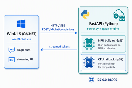
The number that changes the conversation Most "run an LLM locally" tutorials start with the model. This one starts with a bill. Every token a cloud LLM generates is metered. One request is rounding-error cheap. But agents don't make one request — they make thousands, in loops, with retries, across every user, every day, forever. The cost curve of a successful AI feature is not flat; it bends upward with adoption. The thing that makes your product popular is the same thing that makes it expensive to run. That's the uncomfortable truth behind token economics: in the cloud, the marginal cost of intelligence never reaches zero. You rent it, per token, for as long as the feature lives. Edge inference flips the equation. Once the model runs on hardware the user already owns, the marginal cost of the next token trends toward zero. You pay a fixed cost once — the silicon — and then you generate as many tokens as you like. For a whole class of workloads — chat assistants, summarizers, classifiers, on-device copilots — that is a structurally different cost model, and it's the reason "where does inference run" has quietly become one of the most important architecture decisions you'll make this year. To keep this concrete, we'll ground every idea in a real, working repository: kinfey/winml-qwen3-chat — an end-to-end project that builds Qwen3-0.6B for a Windows NPU using Windows ML CLI, benchmarks it against the CPU, and ships a desktop chat app that streams from it token by token. Why the edge — beyond just the bill Cost is the headline, but it's not the whole story. Moving inference onto the device buys you four things at once: Cost. The marginal token approaches free. No per-request metering, no surprise invoice when a feature goes viral. Latency. No network round-trip. The model is a function call away, not an HTTPS request away — and for interactive chat, that's the difference between "snappy" and "spinner." Privacy. The prompt never leaves the machine. For regulated data, personal documents, or anything a user wouldn't paste into a public box, "it never left the laptop" is the strongest guarantee you can offer. Availability. It works on a plane, in a tunnel, behind a corporate firewall, during an outage. Offline isn't a degraded mode — it's the default. The catch has always been: CPUs are bad at this. A general-purpose CPU runs a transformer forward pass slowly and, worse, inconsistently — latency jitters as the OS juggles cores. That's where the silicon story begins. The NPU: purpose-built for the forward pass A modern AI PC has three compute units, and Windows ML exposes each through its own execution provider: Unit Reference silicon (Snapdragon X Elite) Execution Provider NPU Qualcomm Hexagon NPU (X1E80100) QNNExecutionProvider GPU Qualcomm Adreno X1-85 DmlExecutionProvider CPU Snapdragon X 12-core @ 3.40 GHz CPUExecutionProvider The NPU (Neural Processing Unit) is not a faster CPU — it's a different kind of processor, designed for exactly one job: the dense, repetitive matrix multiplication that is model inference. Where a CPU is a brilliant generalist, an NPU is a specialist that does the transformer math at high throughput, low power, and — critically — low variance. That last property matters more than people expect. For an interactive assistant, predictable latency is often worth more than peak latency. A response that always lands in ~1 second feels better than one that averages 0.8s but occasionally stalls for 5. We'll see this show up hard in the benchmark below: the NPU isn't just faster than the CPU here, it's an order of magnitude more consistent. NPUs also sip power. Running inference on the Hexagon NPU instead of pinning twelve CPU cores at 100% means the fan stays quiet and the battery survives the afternoon — which, for an always-available on-device copilot, is the whole point. WinML CLI: from source model to hardware-optimized artifact Here's the gap the NPU story usually hides: a Hugging Face checkpoint does not run on an NPU as-is. You can't hand model.safetensors to the Hexagon and expect tokens. Between "PyTorch weights" and "running on the NPU" sits a real pipeline — export to ONNX, optimize the graph, quantize to integer precision, and compile to a vendor-specific context binary. That pipeline is exactly what Windows ML CLI automates. In its own words, it takes you "from a source model — whether from Hugging Face or your own pipeline — to a hardware-optimized artifact in a reproducible workflow," handling conversion, graph optimization, and compilation across AMD, Intel, NVIDIA, and Qualcomm targets. You can drive each stage by hand (export → analyze → optimize → quantize → compile) or let winml build generate the whole config for you. The same commands target every Windows ML execution provider, so you build once and run across hardware. It's a single CLI, installed as a Python wheel, and it slots cleanly into CI/CD — which is what makes the whole edge-deployment workflow reproducible instead of a one-off science experiment. Walkthrough: building Qwen3-0.6B for the NPU This is the heart of the winml-qwen3-chatt repo. Five steps: install, inspect, build, benchmark, run. 0. Prerequisites The build was validated on a Snapdragon X Elite (ARM64) machine running Windows 11 24H2 (24H2 is required for NPU support), with Python 3.11, the uv package manager, and — for the demo app — the .NET 10 SDK with the WinUI workload. 1. Install the CLI WinML CLI ships on PyPI. Set up an isolated environment with uv and install: # Pin the exact Python the project needs uv python install 3.11 # Create and activate a 3.11 virtual environment uv venv --python 3.11 winml-env .\winml-env\Scripts\activate # Install the CLI from PyPI uv pip install winml-cli # Verify winml --version # -> winml, version 0.1.0 Then let the CLI introspect your machine — this is your first sanity check that the NPU is even visible: winml sys On the reference device this enumerates all three compute units in priority order (NPU → GPU → CPU) and the execution providers behind them (QNNExecutionProvider, DmlExecutionProvider, CPUExecutionProvider). If your NPU doesn't appear here, nothing downstream will use it — winml sys is where you diagnose that. 2. Inspect before you build 💡 Always inspect before build. It catches unsupported architectures in seconds instead of twenty minutes into a failed export. winml inspect -m Qwen/Qwen3-0.6B For Qwen3-0.6B this reports the shape of what you're about to build: a text-generation model mapped to the WinML class WinMLModelForCausalLM (composite), architecture Qwen3ForCausalLM with 28 layers, hidden size 1024, vocabulary 151,936, opset 17. Its inputs are input_ids, attention_mask, and position_ids; its output is logits. One subtlety worth internalizing early: Qwen3 is a composite model — it exports as multiple ONNX components rather than a single graph. That detail comes back to bite you (productively) at quantization time. 3. Build for the NPU This is the one command that does the heavy lifting — export, optimize, quantize, and compile, all targeting the NPU via the QNN execution provider: winml build -m Qwen/Qwen3-0.6B -o output\qwen3-0.6b --ep qnn --device npu --compile -v Under the hood it runs four stages. On the reference device: Stage Time Output Export 133.2 s export.onnx (2.9 GB) Optimize 157.6 s optimized.onnx (2.9 GB) Quantize 227.6 s quantized.onnx (868 MB) — uint8 weight / uint16 activation Compile 437.8 s QNN HTP context (compiled_qnn.bin, 913 MB) Total ~1191.5 s (~20 min) model.onnx + winml_build_config.json The arc of those four rows is the edge-deployment story in miniature: a 2.9 GB float export is quantized down to 868 MB (the integer precision the NPU wants), then compiled into a Qualcomm HTP context binary — a graph the Hexagon NPU can execute directly. The final deployable is output\qwen3-0.6b\model.onnx, a composite entry graph that points at the compiled context. (The ~9 GB of intermediate .onnx.data shards are safe to delete afterward to reclaim disk.) One honest caveat the repo documents: because text-generation isn't in the CLI's built-in calibration task list, quantization falls back to a RandomDataset for calibration. For a latency benchmark that's expected and harmless — but hold that thought, because it's exactly the seam the demo app has to patch for production quality. 4. Benchmark: NPU vs CPU Point winml perf at the compiled model and tell it the task: # NPU (QNN) — runs the compiled context winml perf -m output\qwen3-0.6b\model.onnx --task text-generation --ep qnn --device npu --iterations 100 --warmup 10 # CPU — the compiled NPU graph can't run on CPU, so benchmark the # pre-compile quantized.onnx (QDQ) instead winml perf -m output\qwen3-0.6b\quantized.onnx --task text-generation --ep cpu --device cpu --iterations 50 --warmup 5 The results, for a full prefill forward pass at sequence length 1024: Device EP Precision Avg latency Throughput Std dev NPU QNN w16a16 960.8 ms 1.04 samp/s 3.4 ms CPU CPU w8a16 5793.3 ms 0.17 samp/s 828.3 ms Two takeaways, and the second is the one to remember: The NPU is ~6× faster than the CPU on this workload. The NPU is ~240× more consistent — a 3.4 ms standard deviation versus 828 ms on the CPU. The CPU's latency swings by nearly a full second run to run; the NPU lands in the same spot every time. For an interactive chat experience, that stability is the feature. This is the token-economics argument made physical: the same model, on hardware the user already owns, delivering cloud-grade interactivity at a marginal token cost approaching zero — and doing it more predictably than the CPU fallback ever could. 5. From artifact to app A compiled .onnx isn't a product. The repo closes that gap with a complete desktop example that consumes the NPU build above: app/WinMLChat/ — a WinUI 3 chat UI (C# / .NET 10, MVVM) that streams replies token by token, so the NPU's low, steady latency translates directly into a responsive typing-style experience. backend/ — a FastAPI server exposing an OpenAI-compatible streaming API, backed by winml.modelkit.WinMLAutoModel. The most interesting design decision lives in the backend: hybrid NPU/CPU routing. Short prompts go to the quantized NPU build for speed and efficiency; long prompts fall back to an unquantized CPU path. Conceptually, the routing looks like this: # Illustrative — the backend picks an execution path per request def choose_backend(prompt_tokens: int): if prompt_tokens <= NPU_PREFILL_LIMIT: return npu_model # quantized w16a16, QNN -> fast, low-power return cpu_model # unquantized fallback -> handles long context Because the API speaks the OpenAI streaming dialect, the WinUI front end (and any other OpenAI-compatible client) connects without bespoke glue — the NPU is hidden behind a familiar /chat/completions-style contract. The production seam: patching quantization for a composite decoder Remember the RandomDataset calibration warning? That's the honest boundary between a benchmark and a shipping app, and the repo confronts it head-on. WinML CLI 0.1.0 can't quantize the Qwen3 composite decoder for QNN out of the box — its calibration reader omits position_ids and the 28 layers' past-KV inputs, so the calibration data doesn't match what the model actually consumes at runtime. The example fixes this at the root in backend/winml_npu_patch.py, which: supplies real KV-cache calibration feeds (the actual position_ids and per-layer past-key/value tensors the decoder expects), and switches to per-channel w16a16 weights with the lm_head excluded from quantization. That's the difference between a model that benchmarks well and a model that generates well: calibrating against representative inputs — not random noise — and keeping the precision-sensitive output projection in higher precision so token quality holds up. Where this is still rough It would be dishonest to end on a victory lap. This is early, and it shows. Qwen3-0.6B — and small LLMs in general — aren't enough on their own yet. A 0.6B model is a fine proof point for the pipeline, but it is a modest reasoner. For many real tasks you'll want a larger on-device model, retrieval, or a hybrid edge/cloud design — the silicon is ready before the small-model quality fully is. Performance and optimization still have headroom. The build path works end to end, but there are sharp edges: text-generation falls back to a RandomDataset for calibration, the composite decoder needs a hand-written patch to quantize correctly, operator-level profiling (--op-tracing) isn't available in winml-cli 0.1.0, and the throughput numbers here are a starting line, not a ceiling. Expect to tune. None of this is a reason to wait — it's a reason to get involved. The tooling is open and moving fast, and the fastest way to make it better is to push on it and report what breaks. Found a bug, hit a wall, or have an idea? File it at github.com/microsoft/winml-cli/issues — feedback from real builds is exactly what sharpens these edges. Wrap-up The reason to care about edge AI isn't novelty — it's economics and physics, and they happen to point the same direction. Token economics says the cloud's per-token meter never reaches zero, while the edge drives the marginal token toward free after a one-time hardware cost. For high-volume, interactive, privacy-sensitive workloads, that's a structural advantage, not a rounding error. The NPU is the silicon that makes it viable: purpose-built for the transformer forward pass, delivering — in this build — roughly 6× the CPU's speed and ~240× its consistency, at a fraction of the power. WinML CLI is the bridge that turns a Hugging Face checkpoint into a deployable, hardware-optimized artifact through one reproducible pipeline — inspect → build → perf — that targets every Windows ML execution provider. winml-qwen3-chat ties it all together: a real Qwen3-0.6B NPU build, an honest benchmark, a streaming WinUI app, an OpenAI-compatible backend with hybrid routing, and — most instructively — a quantization patch that shows what it actually takes to move from "runs" to "ships." The headline for builders: inference location is now an architecture decision. When the workload is high-volume, latency-sensitive, or privacy-bound, the right answer increasingly isn't a bigger cloud bill — it's the NPU already sitting in your users' laptops. The tooling to reach it is here today. Start here: Sample Code kinfey/winml-qwen3-chat WinML CLI microsoft/winml-cli654Views2likes0CommentsBuilding an Offline AI Interview Coach with Foundry Local, RAG, and SQLite
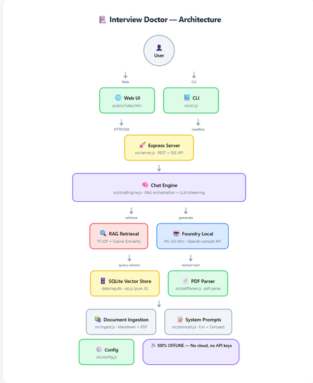
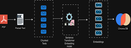
How to build a 100% offline, AI-powered interview preparation tool using Microsoft Foundry Local, Retrieval-Augmented Generation, and nothing but JavaScript. Foundry Local 100% Offline RAG + TF-IDF JavaScript / Node.js Contents Introduction What is RAG and Why Offline? Architecture Overview Setting Up Foundry Local Building the RAG Pipeline The Chat Engine Dual Interfaces: Web & CLI Testing Adapting for Your Own Use Case What I Learned Getting Started Introduction Imagine preparing for a job interview with an AI assistant that knows your CV inside and out, understands the job you're applying for, and generates tailored questions, all without ever sending your data to the cloud. That's exactly what Interview Doctor does. Interview Doctor's web UI, a polished, dark-themed interface running entirely on your local machine. In this post, I'll walk you through how I built an interview prep tool as a fully offline JavaScript application using: Foundry Local — Microsoft's on-device AI runtime SQLite — for storing document chunks and TF-IDF vectors RAG (Retrieval-Augmented Generation) — to ground the AI in your actual documents Express.js — for the web server Node.js built-in test runner — for testing with zero extra dependencies No cloud. No API keys. No internet required. Everything runs on your machine. What is RAG and Why Does It Matter? Retrieval-Augmented Generation (RAG) is a pattern that makes AI models dramatically more useful for domain-specific tasks. Instead of relying solely on what a model learned during training (which can be outdated or generic), RAG: Retrieves relevant chunks from your own documents Augments the model's prompt with those chunks as context Generates a response grounded in your actual data For Interview Doctor, this means the AI doesn't just ask generic interview questions, it asks questions specific to your CV, your experience, and the specific job you're applying for. Why Offline RAG? Privacy is the obvious benefit, your CV and job applications never leave your device. But there's more: No API costs — run as many queries as you want No rate limits — iterate rapidly during your prep Works anywhere — on a plane, in a café with bad Wi-Fi, anywhere Consistent performance — no cold starts, no API latency Architecture Overview Complete architecture showing all components and data flow. The application has two interfaces (CLI and Web) that share the same core engine: Document Ingestion — PDFs and markdown files are chunked and indexed Vector Store — SQLite stores chunks with TF-IDF vectors Retrieval — queries are matched against stored chunks using cosine similarity Generation — relevant chunks are injected into the prompt sent to the local LLM Step 1: Setting Up Foundry Local First, install Foundry Local: # Windows winget install Microsoft.FoundryLocal # macOS brew install microsoft/foundrylocal/foundrylocal The JavaScript SDK handles everything else — starting the service, downloading the model, and connecting: import { FoundryLocalManager } from "foundry-local-sdk"; import { OpenAI } from "openai"; const manager = new FoundryLocalManager(); const modelInfo = await manager.init("phi-3.5-mini"); // Foundry Local exposes an OpenAI-compatible API const openai = new OpenAI({ baseURL: manager.endpoint, // Dynamic port, discovered by SDK apiKey: manager.apiKey, }); ⚠️ Key Insight Foundry Local uses a dynamic port never hardcode localhost:5272 . Always use manager.endpoint which is discovered by the SDK at runtime. Step 2: Building the RAG Pipeline Document Chunking Documents are split into overlapping chunks of ~200 tokens. The overlap ensures important context isn't lost at chunk boundaries: export function chunkText(text, maxTokens = 200, overlapTokens = 25) { const words = text.split(/\s+/).filter(Boolean); if (words.length <= maxTokens) return [text.trim()]; const chunks = []; let start = 0; while (start < words.length) { const end = Math.min(start + maxTokens, words.length); chunks.push(words.slice(start, end).join(" ")); if (end >= words.length) break; start = end - overlapTokens; } return chunks; } Why 200 tokens with 25-token overlap? Small chunks keep retrieved context compact for the model's limited context window. Overlap prevents information loss at boundaries. And it's all pure string operations, no dependencies needed. TF-IDF Vectors Instead of using a separate embedding model (which would consume precious memory alongside the LLM), we use TF-IDF, a classic information retrieval technique: export function termFrequency(text) { const tf = new Map(); const tokens = text .toLowerCase() .replace(/[^a-z0-9\-']/g, " ") .split(/\s+/) .filter((t) => t.length > 1); for (const t of tokens) { tf.set(t, (tf.get(t) || 0) + 1); } return tf; } export function cosineSimilarity(a, b) { let dot = 0, normA = 0, normB = 0; for (const [term, freq] of a) { normA += freq * freq; if (b.has(term)) dot += freq * b.get(term); } for (const [, freq] of b) normB += freq * freq; if (normA === 0 || normB === 0) return 0; return dot / (Math.sqrt(normA) * Math.sqrt(normB)); } Each document chunk becomes a sparse vector of word frequencies. At query time, we compute cosine similarity between the query vector and all stored chunk vectors to find the most relevant matches. SQLite as a Vector Store Chunks and their TF-IDF vectors are stored in SQLite using sql.js (pure JavaScript — no native compilation needed): export class VectorStore { // Created via: const store = await VectorStore.create(dbPath) insert(docId, title, category, chunkIndex, content) { const tf = termFrequency(content); const tfJson = JSON.stringify([...tf]); this.db.run( "INSERT INTO chunks (...) VALUES (?, ?, ?, ?, ?, ?)", [docId, title, category, chunkIndex, content, tfJson] ); this.save(); } search(query, topK = 5) { const queryTf = termFrequency(query); // Score each chunk by cosine similarity, return top-K } } 💡 Why SQLite for Vectors? For a CV plus a few job descriptions (dozens of chunks), brute-force cosine similarity over SQLite rows is near-instant (~1ms). No need for Pinecone, Qdrant, or Chroma — just a single .db file on disk. Step 3: The RAG Chat Engine The chat engine ties retrieval and generation together: async *queryStream(userMessage, history = []) { // 1. Retrieve relevant CV/JD chunks const chunks = this.retrieve(userMessage); const context = this._buildContext(chunks); // 2. Build the prompt with retrieved context const messages = [ { role: "system", content: SYSTEM_PROMPT }, { role: "system", content: `Retrieved context:\n\n${context}` }, ...history, { role: "user", content: userMessage }, ]; // 3. Stream from the local model const stream = await this.openai.chat.completions.create({ model: this.modelId, messages, temperature: 0.3, stream: true, }); // 4. Yield chunks as they arrive for await (const chunk of stream) { const content = chunk.choices[0]?.delta?.content; if (content) yield { type: "text", data: content }; } } The flow is straightforward: vectorize the query, retrieve with cosine similarity, build a prompt with context, and stream from the local LLM. The temperature: 0.3 keeps responses focused — important for interview preparation where consistency matters. Step 4: Dual Interfaces — Web & CLI Web UI The web frontend is a single HTML file with inline CSS and JavaScript — no build step, no framework, no React or Vue. It communicates with the Express backend via REST and SSE: File upload via multipart/form-data Streaming chat via Server-Sent Events (SSE) Quick-action buttons for common follow-up queries (coaching tips, gap analysis, mock interview) The setup form with job title, seniority level, and a pasted job description — ready to generate tailored interview questions. CLI The CLI provides the same experience in the terminal with ANSI-coloured output: npm run cli It walks you through uploading your CV, entering the job details, and then generates streaming questions. Follow-up questions work interactively. Both interfaces share the same ChatEngine class, they're thin layers over identical logic. Edge Mode For constrained devices, toggle Edge mode to use a compact system prompt that fits within smaller context windows: Edge mode activated, uses a minimal prompt for devices with limited resources. Step 5: Testing Tests use the Node.js built-in test runner, no Jest, no Mocha, no extra dependencies: import { describe, it } from "node:test"; import assert from "node:assert/strict"; describe("chunkText", () => { it("returns single chunk for short text", () => { const chunks = chunkText("short text", 200, 25); assert.equal(chunks.length, 1); }); it("maintains overlap between chunks", () => { // Verifies overlapping tokens between consecutive chunks }); }); npm test Tests cover the chunker, vector store, config, prompts, and server API contract, all without needing Foundry Local running. Adapting for Your Own Use Case Interview Doctor is a pattern, not just a product. You can adapt it for any domain: What to Change How Domain documents Replace files in docs/ with your content System prompt Edit src/prompts.js Chunk sizes Adjust config.chunkSize and config.chunkOverlap Model Change config.model — run foundry model list UI Modify public/index.html — it's a single file Ideas for Adaptation Customer support bot — ingest your product docs and FAQs Code review assistant — ingest coding standards and best practices Study guide — ingest textbooks and lecture notes Compliance checker — ingest regulatory documents Onboarding assistant — ingest company handbooks and processes What I Learned Offline AI is production-ready. Foundry Local + small models like Phi-3.5 Mini are genuinely useful for focused tasks. You don't need vector databases for small collections. SQLite + TF-IDF is fast, simple, and has zero infrastructure overhead. RAG quality depends on chunking. Getting chunk sizes right for your use case is more impactful than the retrieval algorithm. The OpenAI-compatible API is a game-changer. Switching from cloud to local was mostly just changing the baseURL . Dual interfaces are easy when you share the engine. The CLI and Web UI are thin layers over the same ChatEngine class. ⚡ Performance Notes On a typical laptop (no GPU): ingestion takes under 1 second for ~20 documents, retrieval is ~1ms, and the first LLM token arrives in 2-5 seconds. Foundry Local automatically selects the best model variant for your hardware (CUDA GPU, NPU, or CPU). Getting Started git clone https://github.com/leestott/interview-doctor-js.git cd interview-doctor-js npm install npm run ingest npm start # Web UI at http://127.0.0.1:3000 # or npm run cli # Interactive terminal The full source code is on GitHub. Star it, fork it, adapt it — and good luck with your interviews! Resources Foundry Local — Microsoft's on-device AI runtime Foundry Local SDK (npm) — JavaScript SDK Foundry Local GitHub — Source, samples, and documentation Local RAG Reference — Reference RAG implementation Interview Doctor (JavaScript) — This project's source codePose Estimation with the AI Dev Gallery
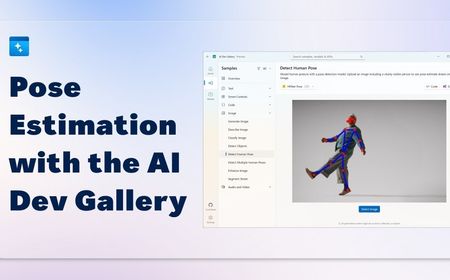
What's Going On Here? This blog post is the first in an upcoming series that will spotlight the local AI samples contained in the new AI Dev Gallery. The Gallery is a preview project that aims to showcase local AI scenarios on Windows and to give developers the guidance they need to enable those scenarios themselves. The Gallery is open-source and contains a wide selection of different models and samples, including text, image, audio, and video use cases. In addition to being able to see a given model in action, each sample contains a source code view and a button to export the sample directly to a new Visual Studio project. The Gallery is available on the Microsoft Store and is entirely open sourced on GitHub. For this first sample spotlight, we will be taking a look at one of my favorite scenarios: Human Pose Estimation with HRNet. This sample is enabled by ONNX Runtime, and depending on the processor in your Windows device, this sample supports running on the CPU and NPU. I'll cover how to check which hardware is supported and how to switch between them later in the post. Pose Estimation Demo This sample takes in an uploaded photo and renders pose estimations onto the main human figure in the photo. It will render connections between the torso and limbs, along with five points corresponding to key facial features (eyes, nose, and ears). Before diving into the code for this sample, here's a quick video example: Let's get right to the code to see how this implemented. Code Walkthrough This walkthrough will focus on essential code and may gloss over some UI logic and helper functions. The full code for this sample can be browsed in depth in the AI Dev Gallery itself or in the GitHub repository. When this sample is first opened, it will make an initial call to LoadModelAsync which looks like this: protected override async Task LoadModelAsync(SampleNavigationParameters sampleParams) { // Tell our inference session where our model lives and which hardware to run it on await InitModel(sampleParams.ModelPath, sampleParams.HardwareAccelerator); sampleParams.NotifyCompletion(); // Make first call to inference once model is loaded await DetectPose(Path.Join(Windows.ApplicationModel.Package.Current.InstalledLocation.Path, "Assets", "pose_default.png")); } In this function, a ModelPath and HardwareAccelerator are passed into our InitModel function, which handles instantiating an ONNX Runtime InferenceSession with our model location and the hardware that inference will be performed on. You can jump to Switching to NPU Execution later in this post for more in depth information on how the InferenceSession is instantiated. Once the model has finished initializing, this function calls for an initial round of inference via DetectPose on a default image. Preprocessing, Calling For Inference, and Postprocessing Output The inference logic, along with the required preprocessing and postprocessing, takes place in the DetectPose function. This is a pretty long function, so let's go through it piece by piece. First, this function checks that it was passed a valid file path and performs some updates to our XAML: private async Task DetectPose(string filePath) { // Check if the passed in file path exists, and return if not if (!Path.Exists(filePath)) { return; } // Update XAML to put the view into the "Loading" state Loader.IsActive = true; Loader.Visibility = Visibility.Visible; UploadButton.Visibility = Visibility.Collapsed; DefaultImage.Source = new BitmapImage(new Uri(filePath)); Next, the input image is loaded into a Bitmap and then resized to the expected input size of the HRNet model (256x192) with the helper function ResizeBitmap: // Load bitmap from image filepath using Bitmap originalImage = new(filePath); // Store expected input dimensions in variables, as these will be used later int modelInputWidth = 256; int modelInputHeight = 192; // Resize Bitmap to expected dimensions with ResizeBitmap helper using Bitmap resizedImage = BitmapFunctions.ResizeBitmap(originalImage, modelInputWidth, modelInputHeight); Once the image is stored in a bitmap of the proper size, we create a Tensor of dimensionality 1x3x192x256 that will represent the image. Each dimension, in order, corresponds to these values: Batch Size: our first value of 1 is just the number of inputs that are being processed. This implementation processes a single image at a time, so the batch size is just one. Color Channels: The next dimension has a value of 3 and corresponds to each of the typical color channels: red, green, and blue. This will define the color of each pixel in the image. Width: The next value of 256 (passed as modelInputWidth) is the pixel width of our image. Height: The last value of 192 (passed as modelInputHeight) is the pixel height of our image. Taken as a whole, this tensor represents a single image where each pixel in that image is defined by an X (width) and Y (height) pixel value and three-color values (red, green, blue). Also, it is good to note that the processing and inference section of this function is being ran in a Task to prevent the UI from becoming blocked: // Run our processing and inference logic as a Task to prevent the UI from being blocked var predictions = await Task.Run(() => { // Define a tensor that represents every pixel of a single image Tensor<float> input = new DenseTensor<float>([1, 3, modelInputWidth, modelInputHeight]); To improve the quality of the input, instead of just passing in the original pixel values to the tensor, the pixels values are normalized with the PreprocessBitmapWithStdDev helper function. This function uses the mean of each RGB value and the standard deviation (how far a value typically varies away from its mean) to "level out" outlier color values. You can think of it as a way of preventing images with really dramatic color differences from confusing the model. This step does not affect the dimensionality of the input. It only adjusts the values that will be stored in the tensor: // Normalize our input and store it in the "input" tensor. Dimension is still 1x3x256x192 input = BitmapFunctions.PreprocessBitmapWithStdDev(resizedImage, input); There is one last small step of set up before the input is passed to the InferenceSession, as ONNX expects a certain input format for inference. A List of type NamedOnnxValue is created with only one entry representing the input tensor that was just processed. Each NamedOnnxValue expects a metadata name (which is grabbed from the model itself using the InferenceSession) and a value (the tensor that was just processed): // Snag the input metadata name from the inference session var inputMetadataName = _inferenceSession!.InputNames[0]; // Create a list of NamedOnnxValues, with one entry var onnxInputs = new List<NamedOnnxValue> { // Call NamedOnnxValue.CreateFromTensor and pass in input metadata name and input tensor NamedOnnxValue.CreateFromTensor(inputMetadataName, input) }; The onnxInputs list that was just created is passed to InferenceSession.Run. It returns a collection of DisposableNamedOnnxValues to be processed: // Call Run to perform inference using IDisposableReadOnlyCollection<DisposableNamedOnnxValue> results = _inferenceSession!.Run(onnxInputs); The output of the HRNet model is a bit more verbose than a list of coordinates that correspond with human pose key points (like left knee, or right shoulder). Instead of exact predictions, it returns a heatmap for every pose key point that scores each location on the image with a probability that a certain joint exists there. So, there's a bit more work to do to get points that can be placed on an image. First, the function sets up the necessary values for post processing: // Fetch the heatmaps list from the inference results var heatmaps = results[0].AsTensor<float>(); // Get the output name from the inference session var outputName = _inferenceSession!.OutputNames[0]; // Use the output name to get the dimensions of the output from the inference session var outputDimensions = _inferenceSession!.OutputMetadata[outputName].Dimensions; // Finally, get the output width and height from those dimensions float outputWidth = outputDimensions[2]; float outputHeight = outputDimensions[3]; The output width and height are passed, along with the heatmaps list and the original image dimensions, to the PostProcessResults helper function. This function does two actions with each heatmap: It iterates over every value in the heatmap to find the coordinates where the probability is highest for each pose key point. It scales that value back to the size of the original image, since it was changed when it was passed into inference. This is why the original image dimensions were passed. From this function, a list of tuples containing the X and Y location of each key point is returned, so that they can be properly rendered onto the image: // Post process heatmap results to get key point coordinates List<(float X, float Y)> keypointCoordinates = PoseHelper.PostProcessResults(heatmaps, originalImage.Width, originalImage.Height, outputWidth, outputHeight); // Return those coordinates from the task return keypointCoordinates; }); Next up is rendering. Rendering Pose Predictions Rendering is handled by the RenderPredictions helper function which takes in the original image, the predictions that were generated, and a marker ratio to define how large to draw the predictions on the image. Note that this code is still being called from the DetectPose function: using Bitmap output = PoseHelper.RenderPredictions(originalImage, predictions, .02f); Rendering predictions is pretty key to the pose estimation flow, so let's dive into this function. This function will draw two things: Red ellipses at each pose key point (right knee, left eye, etc.) Blue lines connecting joint key points (right knee to right ankle, left shoulder to left elbow, etc.) Face key points (eyes, nose, ears) do not have any connections, and will just have dots ellipses rendered for them. The first thing the function does is set up the Graphics, Pen, and Brush objects necessary for drawing: public static Bitmap RenderPredictions(Bitmap image, List<(float X, float Y)> keypoints, float markerRatio, Bitmap? baseImage = null) { // Create a graphics object from the image using (Graphics g = Graphics.FromImage(image)) { // Average out width and height of image. // Ignore baseImage portion, it is used by another sample. var averageOfWidthAndHeight = baseImage != null ? baseImage.Width + baseImage.Height : image.Width + image.Height; // Get the marker size from the average dimension value and the marker ratio int markerSize = (int)(averageOfWidthAndHeight * markerRatio / 2); // Create a Red brush for the keypoints and a Blue pen for the connections Brush brush = Brushes.Red; using Pen linePen = new(Color.Blue, markerSize / 2); Next, a list of (int, int) tuples is instantiated that represents each connection. Each tuple has a StartIdx (where the connection starts, like left shoulder) and an EndIdx (where the connection ends, like left elbow). These indexes are always the same based on the output of the pose model and move from top to bottom on the human figure. As a result, you'll notice that indexes 0-4 are skipped, as those indexes represent the face key points, which don't have any connections: // Create a list of index tuples that represents each pose connection, face key points are excluded. List<(int StartIdx, int EndIdx)> connections = [ (5, 6), // Left shoulder to right shoulder (5, 7), // Left shoulder to left elbow (7, 9), // Left elbow to left wrist (6, 8), // Right shoulder to right elbow (8, 10), // Right elbow to right wris (11, 12), // Left hip to right hip (5, 11), // Left shoulder to left hip (6, 12), // Right shoulder to right hip (11, 13), // Left hip to left knee (13, 15), // Left knee to left ankle (12, 14), // Right hip to right knee (14, 16) // Right knee to right ankle ]; Next, for each tuple in that list, a blue line represenating a connection is drawn on the image with DrawLine. It takes in the Pen that was created, along with start and end coordinates from the keypoints list that was passed into the function: // Iterate over connections with a foreach loop foreach (var (startIdx, endIdx) in connections) { // Store keypoint start and end values in tuples var (startPointX, startPointY) = keypoints[startIdx]; var (endPointX, endPointY) = keypoints[endIdx]; // Pass those start and end coordinates, along with the Pen, to DrawLine g.DrawLine(linePen, startPointX, startPointY, endPointX, endPointY); } Next, the exact same thing is done for the red ellipses representing the keypoints. The entire keypoints list is iterated over because every key point gets an indicator regardless of whether or not it was included in a connection. The red ellipses are drawn second as they should be rendered on top of the blue lines representing connections: // Iterate over keypoints with a foreach loop foreach (var (x, y) in keypoints) { // Draw an ellipse using the red brush, the x and y coordinates, and the marker size g.FillEllipse(brush, x - markerSize / 2, y - markerSize / 2, markerSize, markerSize); } Now just return the image: return image; Jumping back over to DetectPose, the last thing left to do is to update the UI with the rendered predictions on the image: // Convert the output to a BitmapImage BitmapImage outputImage = BitmapFunctions.ConvertBitmapToBitmapImage(output); // Enqueue all our UI updates to ensure they don't happen off the UI thread. DispatcherQueue.TryEnqueue(() => { DefaultImage.Source = outputImage; Loader.IsActive = false; Loader.Visibility = Visibility.Collapsed; UploadButton.Visibility = Visibility.Visible; }); That's it! The final output looks like this: Switching to NPU Execution This sample also supports running on the NPU, in addition to the CPU, if you have met the correct device requirements. You will need a Windows with device with a Qualcomm NPU to run NPU samples in the Gallery. The easiest way to check if your device is NPU capable is within the Gallery itself. Using the Select Model dropdown, you can see which execution providers are supported on your device: I'm on a device with a Qualcomm NPU, so the Gallery is giving the option to run the sample on both CPU and NPU. How Gallery Samples Handle Switching Between Execution Providers When the pose is selected with specific hardware accelerator, that information is passed to the InitModel function that handles how the inference session is instantiated. It will specify the Qualcomm QNN execution provider that enables NPU execution. It looks like this: private Task InitModel(string modelPath, HardwareAccelerator hardwareAccelerator) { return Task.Run(() => { // Check if we already have an inference session if (_inferenceSession != null) { return; } // Set up ONNX Runtime (ORT) session options object SessionOptions sessionOptions = new(); sessionOptions.RegisterOrtExtensions(); if (hardwareAccelerator == HardwareAccelerator.QNN) // Check if QNN was passed { // Add the QNN execution provider if so Dictionary<string, string> options = new() { { "backend_path", "QnnHtp.dll" }, { "htp_performance_mode", "high_performance" }, { "htp_graph_finalization_optimization_mode", "3" } }; sessionOptions.AppendExecutionProvider("QNN", options); } // Create a new inference session with these sessionOptions, if CPU is selected, they will be default _inferenceSession = new InferenceSession(modelPath, sessionOptions); }); } With this function, an InferenceSession can be instantiated to fit whatever execution provider is passed in that particular situation and then that InferenceSession can be used throughout the sample. What's Next More in-depth coverage of the other samples in the gallery will be released periodically, covering a range of what is possible with local AI on Windows. Stay tuned for more sample breakdowns coming soon. In the meantime, go check out the AI Dev Gallery to explore more samples and models on Windows. If you run into any problems, feel free to open an issue on the GitHub repository. This project is open-sourced and any feedback to help us improve the Gallery is highly appreciated.Building Retrieval Augmented Generation on VSCode & AI Toolkit
LLMs usually have limited knowledge about specific domains. Retrieval Augmented Generation (RAG) helps LLMs be more accurate and give relevant output to specific domains and datasets. We will see how we can do this for local models using AI Toolkit,Getting Started - Generative AI with Phi-3-mini: Running Phi-3-mini in Intel AI PC
In 2024, with the empowerment of AI, we will enter the era of AI PC. On May 20, Microsoft also released the concept of Copilot + PC, which means that PC can run SLM/LLM more efficiently with the support of NPU. We can use models from different Phi-3 family combined with the new AI PC to build a simple personalized Copilot application for individuals. This content will combine Intel's AI PC, use Intel's OpenVINO, NPU Acceleration Library, and Microsoft's DirectML to create a local Copilot.33KViews2likes2CommentsFrom Jev to Your Laptop: Building "System One" Decision Models in ONNX with Mobius
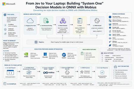
0. Why I'm writing this now Two things landed on my radar in the same week. First, TypeSafe AI published "Introducing System One Models & Jev" (Sep 15, 2026) and the developer community immediately started arguing about it. The pitch is unusual: instead of another chat model, Jev is described as "a new class of frontier models built to make fast, structured decisions that software can use directly." The post frames Jev as "a frontier-intelligence function call: unstructured state in, typed probabilistic decisions out" — and notes that while "Jev gives up string generation, it's optimized for structured outputs and can't hallucinate." The numbers in that post are what got everyone's attention: end-to-end response times of 70ms–500ms versus 3–329 seconds for frontier LLMs, input tokens at $0.042/MTok with output tokens free, and a claim that every answer arrives with a calibrated probability — "higher confidence means higher accuracy." The name itself is a thesis: TypeSafe named Jev after William Stanley Jevons, expecting that "every order of magnitude drop in the cost of intelligence unlocks orders of magnitude more use cases." Second — and this is the part that matters for anyone who builds on Microsoft's AI stack — onnxruntime/mobius has been quietly shipping at a furious pace. It's the piece of infrastructure that makes it realistic to take a model like this, in whatever format it arrives, and run it as an ONNX graph on hardware you control. So I built the bridge. kinfey/JevONNX takes an open, community-fine-tuned model that reproduces the System One request shape, converts it from GGUF to CPU ONNX with Mobius, and serves typed probabilistic decisions locally. This post covers three things: what Mobius is, how it differs from the ONNX Runtime GenAI Model Builder you may already be using, and how the JevONNX sample puts it together. 1. What is Mobius? Mobius builds generative models in ONNX. That preposition is the whole idea. From the repo's own description, Mobius provides "ONNX model definitions for GenAI using the onnxscript.nn API" — model definitions for "LLMs, MoE, multimodal, encoder-only, encoder-decoder, vision, audio, and diffusion models — built directly as ONNX graphs using onnxscript.nn.Module." The key sentence, and the one worth reading twice: "Rather than tracing or exporting PyTorch models, it constructs the ONNX graph declaratively, then applies pretrained HuggingFace weights." Why "declarative construction" is a big deal If you've ever exported a model to ONNX the traditional way, you know the failure modes. You run torch.onnx.export, the tracer executes one concrete path through Python control flow, and anything dynamic — a KV cache branch, a rotary embedding computed with a Python if, a sliding-window mask — either silently bakes in a constant or explodes into an unreadable subgraph. You then spend a week diffing graphs. Mobius inverts this. The graph is the source of truth, written as composable modules, and the weights are applied afterwards. The architecture in the README is four clean layers: HuggingFace Hub │ ▼ ArchitectureConfig ◄── from_transformers() / from_diffusers() │ ▼ Model Module ◄── Reusable Components (Attention, MLP, RMSNorm, RoPE, …) │ ▼ Task ◄── CausalLMTask, VisionLanguageTask, VAETask, DenoisingTask, … │ ▼ ONNX Model ◄── preprocess_weights() + apply_weights() Components — onnxscript.nn.Module building blocks (Attention, MLP, DecoderLayer, RoPE, VisionEncoder, MoELayer…) Models — full architectures composed from those components Tasks — define the ONNX graph's I/O contract (inputs, outputs, KV cache) Registry — maps HuggingFace model_type strings to model classes Adding a new architecture becomes writing a model definition, not debugging an exporter. Mobius even ships developer skills in .agents/skills/ (adding-a-new-model, reusable-components, moe-models, multimodal-models, writing-tests, writing-rewrite-rules) so an AI coding agent can do the legwork with you. Coverage This isn't a toy. The repo claims 290+ Transformers model types and 10 Diffusers component types across 40+ task types and 100+ reusable components, spanning: Category Examples Text generation Llama 2/3/4, Mistral, Qwen 2/2.5/3/3.5/3.6, Phi-3/3.5, Gemma 1/2/3/4, Granite, GPT-2, OPT, OLMo, SmolLM3 Mixture of Experts PhiMoE, GPTOSS, Mixtral, OLMoE, DeepSeek-V2/V3, Qwen2-MoE, Qwen3-MoE, Qwen3-Next, GLM-4-MoE, Arctic, DBRX, Jamba Multimodal Gemma 3/4, Phi-4MM (vision + audio + LoRA), LLaVA, InternVL2, MiniCPM-V 4.6, Qwen2.5-VL, Qwen3-VL, Pixtral Encoder-only BERT, RoBERTa, ALBERT, DeBERTa, DistilBERT, ELECTRA, XLNet Encoder-decoder BART, T5/mT5, Marian, M2M-100, Pegasus, BigBird-Pegasus Speech-to-text Whisper, Moonshine, Moonshine Streaming, FastConformer-RNNT, FunASR, GLM-ASR, Qwen3-ASR, SenseVoice Audio Wav2Vec2, HuBERT, WavLM, SpeechT5 Vision ViT, BEiT, DeiT, DINOv2, Swin, CLIP, SigLIP Diffusion Stable Diffusion (UNet + VAE + ControlNet), Flux, SD3, DiT, QwenImage / Qwen-Image-Edit-2509, HunyuanDiT, CogVideoX Adapters T2I-Adapter, IP-Adapter The five-minute version pip install -e . from mobius import build pkg = build("meta-llama/Llama-3.2-1B") pkg.save("output/llama-3.2-1b/") Static KV cache, when you know your max sequence length up front: from mobius import build, CausalLMTask task = CausalLMTask(static_cache=True, max_seq_len=2048) pkg = build("meta-llama/Llama-3.2-1B", task=task) pkg.save("output/llama-3.2-1b-static/") EP-aware optimization — the graph itself is tuned per execution provider, "each with the right set of fused kernels and lowering passes applied automatically": # CUDA: GQA fusion, SkipLayerNorm, PackQKV pkg = build("meta-llama/Llama-3.2-1B", execution_provider="cuda", dtype="f16") # WebGPU: GQA fusion, Shape ops replaced with portable alternatives pkg = build("meta-llama/Llama-3.2-1B", execution_provider="webgpu", dtype="f16") And the CLI, which is what we'll use later: mobius build --model Qwen/Qwen2.5-0.5B --output output_dir/ mobius build --model meta-llama/Llama-3.2-1B --output output_dir/ --ep cuda --dtype f16 mobius build --model openai/whisper-tiny --output output_dir/ # encoder/ + decoder/ Build-mode toggles use a cargo-style --features flag — available features are static-cache, fp8-kv-cache, prune-prefill-prefix, and text-only: mobius build --model meta-llama/Llama-3.2-1B --output output_dir/ \ --features static-cache,prune-prefill-prefix --max-seq-len 2048 --release strips build-time debug and provenance metadata to reduce saved model size, while preserving functional metadata keyed with the mobius. prefix. 2. Mobius vs. the ONNX Runtime GenAI Model Builder This is the question I get every time I demo Mobius, so let's be precise. Both are Microsoft tools, both produce ONNX, and they are not competitors — they sit at different points on the same pipeline. The ONNX Runtime GenAI Model Builder describes itself as the tool "for quickly creating optimized and quantized ONNX models within a few minutes that run with ONNX Runtime GenAI." Its output is a deployment-ready package: model.onnx plus genai_config.json plus tokenizer files, wired for the onnxruntime-genai runtime. Its architecture list is explicitly curated — AMD OLMo, ChatGLM, DeepSeek, ERNIE 4.5, Gemma, gpt-oss, Granite, Granite MoE Hybrid, HunYuan Dense V1, InternLM2, LFM2, LFM2 MoE, Llama, Mistral, Nemotron, Phi, Qwen, SmolLM3, Whisper — and the README states plainly that "it is intended for supporting the latest, popular state-of-the-art models." Mobius, by contrast, is a model-definition library: a component algebra for describing generative architectures as ONNX graphs, with a registry mapping HuggingFace model_type strings to model classes. Here's how I'd separate them: Dimension ORT GenAI Model Builder Mobius Primary goal Produce a deployment-ready GenAI package, fast Define and construct the ONNX graph itself Output contract model.onnx + genai_config.json + tokenizer, targeted at the ORT GenAI runtime ONNX model package; you choose the runtime (plain ORT sessions included) How the graph is made Per-architecture builder subclasses (LlamaModel, QwenModel, Phi3MiniModel, WhisperModel…) overriding make_layer / make_attention / make_moe Declarative onnxscript.nn.Module composition from reusable Components → Models → Tasks Breadth Curated list of ~19 popular families, text + Whisper 290+ Transformers types, 10 Diffusers component types, 40+ tasks — including vision, audio, and diffusion Extending it Add a builder subclass inside the onnxruntime-genai tree Add a model definition from existing components; shipped .agents/skills/ guide it Tuning surface Rich --extra_options for quantization and runtime behavior (QMoE, paged attention, KV-cache quantization, QDQ, CUDA/WebGPU graph capture…) --features build toggles + execution_provider= EP-aware graph lowering + dtype control Diffusion / multi-component pipelines Not the target First-class (--model Qwen/Qwen-Image-2512 builds all components) When I reach for it "I have a Phi/Llama/Qwen chat model and I want an int4 CPU/CUDA package running under ORT GenAI today" "My architecture is hybrid, unusual, multimodal, diffusion, or I need graph-level control over what gets emitted" Notably, the two overlap on real capabilities. The Model Builder also consumes GGUF and handles Qwen3.5-class features (compact state updates, recurrent-operator selection). Mobius also emits ORT-GenAI-compatible metadata — though the repo is honest about limits: for Mage-VL, "ORT GenAI export is currently rejected because the runtime cannot supply its required patch_positions input or Mage-VL's 1D decoder positions." That single line tells you exactly where the boundary sits: the Model Builder is bounded by what the GenAI runtime can express; Mobius is bounded by what ONNX can express. My rule of thumb as an advocate: if your model is on the Model Builder's supported list and you want the GenAI runtime's generation loop, use the Model Builder — it is faster and gives you a complete package. The moment you're off that list, or you need the graph itself to be a first-class artifact you can reason about and modify, Mobius is the tool. The JevONNX sample is squarely in the second category. Let's look at why. 3. The sample: converting a Jev-style decision model to CPU ONNX Repo: github.com/kinfey/JevONNX 3.1 The honest framing first Jev is TypeSafe's proprietary model. You can't download it and convert it, and this project doesn't pretend otherwise. What the community did do is interesting: n4ze3m/Qwen3.5-4B-Hmm is "an experimental open-model attempt to reproduce the central idea and request shape of the System One workflow introduced with Jev." It works by "fine-tuning Qwen3.5-4B to answer typed questions through option probabilities instead of ordinary generated text." The README of JevONNX is emphatic about the boundaries, and I want to repeat them here rather than bury them: "Hmm is not Jev, is not affiliated with TypeSafe AI, and does not reproduce Jev's proprietary model architecture, parallel sampler, performance, calibration, or type-safety guarantees. The Hmm model card explicitly states that it is less capable than Jev." And: "The reproduction is behavioral rather than architectural." The distinction, straight from the project's comparison table: Property Jev Hmm in this project Model design Native System One Model Qwen3.5-4B fine-tuned to reproduce the typed-decision concept Output mechanism Native typed probabilistic outputs First-token option-letter probabilities Multiple questions Designed for parallel sampling Jev-like request shape, implemented as one model pass per question Output types Schema-constrained structured values noul, choice, and score adapter Runtime here TypeSafe service Local ONNX Runtime CPU Guarantees As documented by TypeSafe No equivalent guarantee is claimed The mechanism is refreshingly legible: the adapter turns each typed question into an exact multiple-choice prompt, then "reads the first generated-token logits for A, B, C, and subsequent option letters and normalizes them into probabilities." No JSON parsing, no retry-on-malformed-output, no regex. The probability distribution is the answer. 3.2 Why this needs Mobius specifically Qwen3.5 is a hybrid architecture, and that's the whole reason this is a Mobius story. The exported model has 32 hybrid decoder layers. Linear-attention layers carry conv_state and recurrent_state; full-attention layers carry key/value caches. In this artifact, full-attention layers sit at indices 3, 7, 11, 15, 19, 23, 27, and 31. The practical consequence, quoted from the README: "The prompt is processed one token at a time while every present.* output is fed back into its corresponding past_key_values.* input. This differs from a conventional decoder-only example that can prefill an entire prompt in one call." That is a graph-shape problem. You cannot handwave it with a config flag — you need the exported graph's state contract to be explicit and inspectable, which is exactly what declarative construction gives you. The implementation "follows the structure of Mobius examples/text_generation.py while adding the hybrid-state handling required by Qwen3.5." 3.3 The conversion pipeline n4ze3m/Qwen3.5-4B-Hmm-Q4_K_M.gguf │ SHA-256 verification ▼ Mobius GGUF reader/importer │ metadata and tensor mapping │ Qwen3.5 hybrid graph construction │ Q4_K_M → packed quantized target storage │ CPU execution-provider optimization ▼ onnx_outputs/ ├── model.onnx ├── model.onnx.data ├── quantization_report.json ├── tokenizer.json ├── tokenizer_config.json ├── chat_template.jinja └── cpu_test_summary.json │ ▼ ONNX Runtime CPUExecutionProvider │ token-by-token hybrid-state prefill │ first-token A/B/C/… probabilities ▼ typed decision JSON response One command does the conversion: mobius build-gguf Qwen3.5-4B-Hmm-Q4_K_M.gguf \ --output onnx_outputs \ --ep cpu \ --dtype f32 \ --release Two details worth internalizing: --dequantize is intentionally not used. Keeping quantized storage "substantially reduc[es] the output size compared with a fully dequantized FP32 model." The external-data file is still ~2.6 GB — imagine it dequantized. Don't trust the preset, read the report. "Q4_K conversion can involve a lossy affine repack; inspect quantization_report.json rather than assuming source-preset fidelity." This is the kind of line that separates a demo from a deployment. 3.4 Reproducibility — the part I actually want you to copy Every pin, in a table, in the README: Component Revision GGUF repository n4ze3m/Qwen3.5-4B-Hmm GGUF revision c27fa3c627dfaced343c6ba9d3a0d00243a3be51 GGUF filename Qwen3.5-4B-Hmm-Q4_K_M.gguf GGUF SHA-256 5e03cb057049c56b421bd3c506d77fd8e0a77996bb8464148a02cfc3caac5229 Mobius revision 6b27a3f08b8b5d08ba9b14b416e3b435942bb0bd Tokenizer repository Qwen/Qwen3.5-4B Tokenizer revision 851bf6e806efd8d0a36b00ddf55e13ccb7b8cd0a The notebook builds a Mobius wheel from the pinned Git source rather than installing a prebuilt package. On a project moving at 500+ commits, that is not paranoia — that is the only way your conversion is still reproducible next month. 3.5 Running it Two files carry the project: Qwen3_5_4B_Hmm_GGUF_to_CPU_ONNX_Mobius_fixed.ipynb (the Colab conversion and validation workflow) and run_hmm_onnx.py (the standalone typed-decision runner). Run the notebook in a high-memory Colab CPU runtime; it writes to /content/onnx_outputs on Colab and .mobius_colab_run/onnx_outputs elsewhere. Then: python run_hmm_onnx.py --model-dir .mobius_colab_run/onnx_outputs python run_hmm_onnx.py --model-dir .mobius_colab_run/onnx_outputs --request request.json A request is state plus typed questions: { "state": "Help! My payouts have failed for 3 days. I need the money today.", "questions": { "is_urgent": { "type": "noul", "instructions": "Does this message convey urgency?" }, "department": { "type": "choice", "instructions": "Which team should handle this?", "criteria": { "billing": "Payments, invoicing, refunds", "technical": "Bugs, outages, integrations", "sales": "Pricing, upgrades, new accounts" } }, "priority": { "type": "score", "instructions": "How urgent is this request?", "criteria": ["Not urgent", "Normal", "Urgent", "Critical"] } } } From Python: from pathlib import Path from run_hmm_onnx import HmmOnnx model = HmmOnnx(Path(".mobius_colab_run/onnx_outputs")) response = model.decide({ "state": "Help! My payouts have failed for 3 days.", "questions": { "is_urgent": { "type": "noul", "instructions": "Does this message convey urgency?", } }, }) print(response) 3.6 The three decision types noul — a nullable-style yes/no probability; the probability of the true option: { "type": "noul", "noul": 0.9745 } choice — the highest-probability key, all normalized option probabilities, and a confidence value measuring how peaked the distribution is: { "type": "choice", "choice": "billing", "probabilities": { "billing": 0.7216, "technical": 0.2759, "sales": 0.0025 }, "confidence": 0.5823 } score — the expected numeric level, the level legend, normalized probabilities, and confidence: { "type": "score", "score": 2.6653, "legend": { "0": "Not urgent", "1": "Normal", "2": "Urgent", "3": "Critical" }, "probabilities": { "0": 0.0061, "1": 0.0361, "2": 0.2443, "3": 0.7135 }, "confidence": 0.618 } Look at that score output for a second. You don't get "this is critical." You get 2.6653 — a distribution leaning hard on Critical but with real mass on Urgent. That's a number your routing code can threshold on, log, and A/B test. It's the difference between an LLM that says it's confident and a distribution you can actually calibrate against. One constraint: Hmm is trained with 26 option letters. Larger option sets are handled by splitting them into groups of 25 and adding a none_of_these option to each group, matching the reference Hmm server strategy. 3.7 Does it actually run? Yes — the README reports the generated model executed directly on an Apple Silicon CPU with ONNX Runtime. A 4B hybrid-architecture model, converted from GGUF, running typed decisions on a laptop CPU with no service dependency. 4. What I'd tell a room of developers The System One idea is portable even where the model isn't. You can't run Jev locally, but the shape — state in, typed decisions with probabilities out — is something you can prototype today with an open model and an ONNX graph. As TypeSafe puts it, structured outputs "slot into ordinary software as fuzzy decision rules: classify, route, score, extract, or branch where hand-written logic is too brittle." That's a pattern, not a product. Probabilities are the actual product. The reason this class of model matters isn't speed alone. TypeSafe's argument is sharp: "If a model can do a task 95% of the time but doesn't say when it's in the 5%, it can't automate that task." Every engineer who has shipped an LLM feature has felt that exact wall. Set expectations honestly. JevONNX is an educational reproduction. It gives you noul/choice/score on a local CPU. It does not give you Jev's calibration, parallel sampler, or type-safety guarantees — and the project says so in its own README. Ship that caveat with your demo. Mobius is the infrastructure bet worth learning. When a new architecture shows up — hybrid attention, a novel MoE routing scheme, a three-model multimodal export — the question stops being "will the exporter support it?" and becomes "which components do I compose?" That is a much better question to be asking. Links Mobius — https://github.com/onnxruntime/mobius (docs: https://onnxruntime.github.io/mobius/) ONNX Runtime GenAI Model Builder — https://github.com/microsoft/onnxruntime-genai/tree/main/src/python/py/models JevONNX sample — https://github.com/kinfey/JevONNX Introducing System One Models & Jev — https://typesafe.ai/blog/introducing-system-one-models-and-jev Hugging face - https://huggingface.co/lokinfey/Qwen3_5_4B_Hmm_ONNXoBeaver — A Beaver That Runs LLMs on Your Machine 🦫
Hi there! I'm the creator of oBeaver. This project started from a pretty simple desire: I wanted to run large language models on my own computer. No data sent to the cloud. No API keys. No per-call charges. I'm guessing you've had the same thought. There are already great tools out there — Ollama being the most prominent. But in my day-to-day work, I spend a lot of time in the ONNX ecosystem — the cross-platform reach of ONNX Runtime, its native NPU support, the turnkey experience of Microsoft Foundry Local. It kept nagging at me: the ONNX ecosystem deserves a more complete local inference toolkit. That's how oBeaver was born. Here are the links if you want to jump straight in: GitHub: https://github.com/microsoft/obeaver Docs: https://microsoft.github.io/obeaver Up and Running in Three Minutes Getting started with oBeaver is dead simple. You need Python 3.12+, then it's clone, install, chat: git clone https://github.com/microsoft/obeaver.git cd obeaver pip install -e . # Initialize the model directory (auto-creates ort/, foundrylocal/, cache_dir/ sub-folders) obeaver init # Make sure everything looks good obeaver check If you're on macOS or Windows, install Foundry Local and you're one command away from chatting with a model: obeaver run phi-4-mini The first run downloads the model automatically — give it a minute. After that, it's instant. On Linux, or if you want to use models from Hugging Face, the ORT engine has you covered: # Convert Qwen3-0.6B from Hugging Face to ONNX format obeaver convert Qwen/Qwen3-0.6B # Run it with the ORT engine obeaver run --engine ort ./models/ort/Qwen3-0.6B_ONNX_INT4_CPU Want to turn your model into an HTTP service? One line: obeaver serve Phi-4-mini Then point any OpenAI-compatible client at it — just change one base_url and your existing code works as-is: from openai import OpenAI client = OpenAI(base_url="http://127.0.0.1:18000/v1", api_key="unused") response = client.chat.completions.create( model="Phi-4-mini", messages=[{"role": "user", "content": "What is the capital of France?"}], stream=True, ) for chunk in response: print(chunk.choices[0].delta.content or "", end="", flush=True) LangChain, LlamaIndex, Microsoft Agent Framework, CrewAI — anything that speaks the OpenAI protocol plugs right in. This was a non-negotiable design principle from day one: local inference shouldn't be an island; it should fit seamlessly into your existing dev workflow. "Why Not Just Use Ollama?" I get this question a lot, and it deserves a straight answer. Ollama is a fantastic project. It pioneered the "one command to run a model" experience and made local LLM inference accessible to everyone. If all you need is a quick way to chat with a model locally, Ollama is still a wonderful choice. oBeaver itself draws heavy inspiration from it. But Ollama and oBeaver take different technical paths. Ollama is built on llama.cpp and uses the GGUF model format. oBeaver is built on ONNX Runtime and uses the ONNX model format. Behind these two formats are two very different philosophies. GGUF: Grab and Go GGUF's strength is ultimate portability. One file bundles everything — weights, tokenizer, metadata. Hugging Face is packed with pre-quantized GGUF models ready to download and run. Quantization options are rich (Q2_K through Q8_0), and the community is incredibly active. For individual developers, this "grab and go" experience is hard to beat. ONNX: Convert Once, Accelerate Everywhere ONNX shines in a different dimension. As a cross-platform industrial standard, ONNX Runtime has something called Execution Providers — the same ONNX model, without any changes, can run on CPU, GPU, and even NPU. This matters more than it might seem at first glance. With chips like Intel Core Ultra, Qualcomm Snapdragon X, and Apple Neural Engine becoming mainstream, NPUs are quickly becoming standard hardware in AI PCs. ONNX Runtime already supports NPU acceleration natively, while the GGUF ecosystem doesn't have this capability yet. This means ONNX naturally adapts to a far wider range of devices — from servers to laptops, from desktops to edge devices, even phones and IoT endpoints. The ONNX model you run on CPU today can be accelerated on an NPU-equipped machine tomorrow — no re-conversion, no code changes, just switch the Execution Provider. ONNX does have a higher barrier to entry — models need to be converted first. But oBeaver's built-in obeaver convert command, powered by Microsoft's Olive toolkit, reduces that to a single line. Another project worth mentioning is oMLX, which also explores local inference in the ONNX ecosystem, but focuses specifically on Apple Silicon. oBeaver aims to be more comprehensive — spanning macOS, Windows, and Linux, covering text chat, embeddings, and vision-language scenarios. Here's a quick comparison of all three: Ollama oMLX oBeaver Model format GGUF ONNX ONNX Inference backend llama.cpp ONNX Runtime Foundry Local + ORT GenAI Platforms macOS/Linux/Windows macOS macOS/Windows/Linux NPU acceleration ❌ ❌ ✅ Embedding models ✅ ✅ ✅ VL models ✅ ✅ ✅ Function Calling ✅ ✅ ✅ Docker deployment ✅ ✅ ✅ I'm not saying oBeaver is better than Ollama. They serve different needs. But if your work involves the ONNX ecosystem, NPU acceleration, or a combination of embedding and multimodal capabilities, oBeaver offers a path that Ollama doesn't currently cover. Why a "Dual Engine"? This is oBeaver's most distinctive design decision, and the one I spent the most time thinking about. oBeaver has two inference engines under the hood: Foundry Local and ONNX Runtime GenAI (ORT). Why not just pick one? Because reality is messier than ideals. Foundry Local is Microsoft's local inference runtime, and the experience is lovely — pass a catalog alias like Phi-4-mini, and it auto-downloads, loads, and runs the model with smart hardware scheduling (NPU > GPU > CPU). But it has two clear limitations: first, the model catalog is still small, mostly centered around Microsoft's Phi family; second, it only supports macOS and Windows — Linux users are left out. ONNX Runtime GenAI fills exactly those gaps. It supports macOS, Windows, and Linux — all three platforms. And with obeaver convert, you can transform almost any model on Hugging Face into ONNX format, giving you a much wider model selection. Right now, oBeaver can already run models from Phi, Qwen, Gemma, GLM, and other SLM families through the ORT engine. On top of that, the ORT engine powers capabilities that Foundry Local simply can't do: Embedding models — The ORT engine includes a dedicated embedding engine supporting Qwen3-Embedding and EmbeddingGemma, perfect for local RAG pipelines: # Start the embedding service obeaver serve-embed ./models/Qwen3-Embedding-0.6B from openai import OpenAI client = OpenAI(base_url="http://127.0.0.1:18001/v1", api_key="unused") response = client.embeddings.create( model="Qwen3-Embedding-0.6B", input=["Hello, world!", "Embeddings are useful."], ) for item in response.data: print(f"index={item.index} dim={len(item.embedding)}") Vision-Language models (VL) — When the ORT engine detects vision.onnx in a model directory, it automatically switches to VL mode. Currently supported: Qwen-2.5-VL-3B and Qwen-3-VL-2B. You can send images alongside text for multimodal understanding: obeaver serve ./models/Qwen3-VL-2B-Instruct_VL_ONNX_INT4_CPU Converting a VL model is just one command too: obeaver convert Qwen/Qwen2.5-VL-3B-Instruct --type vl So the dual engine isn't redundancy — it's the optimal choice given reality: Foundry Local covers only macOS/Windows; ORT GenAI covers all platforms. Foundry Local has fewer models but zero friction; ORT GenAI has more models and more flexibility. oBeaver automatically picks the right engine for your platform and task — Foundry Local by default on macOS/Windows, ORT on Linux, auto-switching to ORT for embedding or VL workloads. You can always override with --engine ort. In short: Foundry Local handles the "just works" path, ORT handles the "I need more" path. Together, they give oBeaver an answer for every platform and every scenario. Cloud-Native? Of Course oBeaver isn't just a local toy. Deployment was baked into the design from the start. The architecture is cleanly layered: CLI (Typer) → FastAPI Server → pluggable inference engines. We ship a Docker image supporting both linux/amd64 and linux/arm64 (Apple Silicon included): # Build the image docker buildx build --platform=linux/amd64 \ -f docker/Dockerfile.cpu -t obeaver-cpu . # Start the API server docker run -d --rm -p 18000:18000 \ -v /path/to/models:/models \ obeaver-cpu serve -m /models -E ort --host 0.0.0.0 --port 18000 Local dev, CI/CD pipelines, headless servers, Kubernetes clusters — it all works. Combined with the OpenAI-compatible API, you can develop against oBeaver locally and switch to a cloud endpoint in production by changing a single URL. Not a single line of application code needs to change. Not Just a CLI — There's a Dashboard Too So far everything I've shown has been terminal commands. But sometimes you just want a visual interface — especially when you're evaluating models, comparing performance, or showing a demo. oBeaver ships with a built-in web dashboard. One command to launch: obeaver dashboard # Foundry Local engine (macOS/Windows) obeaver dashboard -e ort # ORT engine (scans local ONNX models) Open http://127.0.0.1:1573/ and you'll see something like this: It's a real-time monitoring and chat interface rolled into one. Here's what you get: Model Selector — Switch between your cached models on the fly. If a model supports NPU acceleration, it's marked with a ⚡ badge. With Foundry Local, you'll see the models from your local catalog: With the ORT engine, it scans your model directory for all available ONNX models: Chat + Live Benchmarking — Send messages and get streaming responses, with real-time performance stats right in the interface — TTFT (Time to First Token), tokens per second, total token count. This makes it incredibly easy to benchmark different models side by side: System Monitoring — Real-time memory gauges for CPU, GPU, NPU, and process memory. A system info bar shows the current model, engine type, platform, and health status at a glance. Inference Parameters — Adjust temperature, top-p, top-k, and max tokens with built-in presets, all without restarting the server. VL Mode — When you load a Vision-Language model in the ORT dashboard, the interface automatically switches to a dedicated VL mode where you can provide an image URL alongside your text prompt: And more — Conversation history with save/load, system prompt configuration, live server logs showing every request with method/path/status/timing, and export to JSON or Markdown. The dashboard isn't a separate product — it's just obeaver dashboard. Everything runs locally, nothing phones home. It's particularly useful when you want to quickly evaluate how a model performs on your hardware before committing to it in your application. Being Honest: CPU Only for Now oBeaver is currently in Tech Preview, and I want to be upfront about this — it only supports CPU inference right now. This is a deliberate, stage-by-stage choice. We wanted to make sure the entire toolchain — model conversion, inference, API serving, Docker deployment — is rock solid on CPU first. Almost every machine has a CPU; it's the best baseline for validating the complete workflow. But GPU and NPU support are coming soon. They're at the very top of the roadmap. ONNX Runtime already ships mature CUDA (GPU) and QNN/OpenVINO (NPU) Execution Providers. Foundry Local already has NPU > GPU > CPU auto-scheduling built in. What oBeaver needs to do is integrate these into its engine selection logic and model conversion pipeline — and that work is actively underway. Ultimately, one of the key reasons oBeaver chose the ONNX path is the NPU future. The AI PC era is arriving, and when NPUs become standard hardware, ONNX will be the ecosystem most ready for it. Acknowledgements oBeaver is inspired by and builds upon the ideas from the following excellent projects: Project Description Ollama Run large language models locally with a simple CLI OMLX Run large language models on Apple Silicon, ONNX-based vLLM High-throughput and memory-efficient inference engine for LLMs Foundry Local Microsoft's local model inference runtime with NPU/GPU/CPU acceleration ONNX Runtime GenAI Generative AI extensions for ONNX Runtime Olive Microsoft's model optimization toolkit for ONNX Runtime I Need Your Feedback That's the tour. But oBeaver is still in its early days, and there's so much room to improve. As the creator of this project, what I fear most isn't criticism — it's silence. So I genuinely hope you'll give it a try and let me know what you think: Which models do you most want to run? How urgent is GPU / NPU acceleration for your use case? What do you think of the dual-engine design — does it add value, or does it add complexity? In your real-world projects, what's the biggest pain point with local inference? What else does the Docker story need? Helm Charts? Compose files? GitHub Issues, PRs, or just reaching out on social media — any form of feedback is deeply appreciated. The name oBeaver comes from the beaver — nature's most remarkable engineer. Beavers build dams stick by stick, creating the environment they need to thrive. I hope oBeaver can help you do the same: build your local AI infrastructure, one piece at a time, on your own hardware. Build local. Dam the cloud. 🦫 GitHub: https://github.com/microsoft/obeaver Docs: https://microsoft.github.io/obeaver If you find oBeaver useful, a ⭐ on GitHub means the world to us!