ai infrastructure
114 TopicsBuild a Simple GPU-Enabled Kubernetes Cluster on Azure N-Series VMs
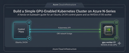
Audience: Platform engineers, ML engineers, and developers who need a small, understandable GPU development cluster without the abstraction of a managed Kubernetes service. Reference topology: Role Azure VM size Operating system Purpose Control plane Standard_D8s_v6 Ubuntu 24.04 LTS API server, scheduler, controllers, etcd GPU worker Standard_NC24ads_A100_v4 Ubuntu 24.04 LTS CUDA-enabled development workloads Software baseline: Kubernetes v1.33, containerd, Flannel CNI, NVIDIA Container Toolkit, and NVIDIA Kubernetes device plugin v0.17.0. Why Build This Cluster? A two-node kubeadm cluster is useful when you want direct access to Kubernetes internals while developing or debugging GPU applications. It keeps the control plane on a general-purpose VM and reserves the expensive N-series capacity for workloads that explicitly request a GPU. Development Use Case: Shared GPU Sandbox Imagine a small ML team validating a PyTorch service before moving it to a production platform. Developers build containers locally or in CI, deploy them to this cluster, request nvidia.com/gpu: 1, inspect CUDA behavior, tune resource requests, and test Kubernetes manifests. The same environment can exercise Jobs, model-serving Deployments, ConfigMaps, Secrets, storage mounts, and observability agents. This design is appropriate for experimentation, integration testing, workshops, and short-lived development. It is not a production blueprint: the control plane is not highly available, etcd has no redundancy, Flannel is intentionally simple, and operational safeguards are minimal. Architecture and Traffic Flow Control plane: runs the Kubernetes API server, scheduler, controller manager, and etcd. GPU worker: runs containerd, kubelet, the NVIDIA container runtime, and GPU workloads. Pod network: Flannel allocates pod addresses from 10.244.0.0/16. GPU discovery: the NVIDIA device plugin advertises nvidia.com/gpu to Kubernetes. Before You Begin Create both VMs in the same Azure virtual network and subnet. Use private IP connectivity between nodes. Confirm that the selected region has quota and capacity for Standard_NC24ads_A100_v4. GPU VM availability and quota are subscription- and region-dependent. Use trusted administrative source ranges for SSH. Ensure the nodes can communicate on the Kubernetes control-plane, kubelet, and Flannel ports required by your network policy. Avoid exposing the Kubernetes API server broadly to the internet. Disk requirement: Use 128GB disk as OS disk in Standard_NC24ads_A100_v4 as 32GB will be the default and it may not be sufficient to run the test job mentioned below. 1. Prepare Both Nodes Run the following commands on both the control-plane VM and the GPU worker. Use a non-root account with sudo access. Set Host Names and Name Resolution Assign a unique host name on each VM: Control plane sudo hostnamectl set-hostname controlplane GPU worker sudo hostnamectl set-hostname gpunode Add both private IP addresses to /etc/hosts on each node, replacing the placeholders: <CONTROL_PLANE_PRIVATE_IP> controlplane <GPU_WORKER_PRIVATE_IP> gpunode Disable Swap Kubelet expects swap to be disabled unless it is explicitly configured to tolerate it. sudo swapoff -a sudo sed -i '/ swap / s/^/#/' /etc/fstab swapon --show The final command should return no active swap devices. Load Required Kernel Modules cat <<EOF | sudo tee /etc/modules-load.d/k8s.conf overlay br_netfilter EOF sudo modprobe overlay sudo modprobe br_netfilter Configure Kubernetes Networking Parameters cat <<EOF | sudo tee /etc/sysctl.d/k8s.conf net.bridge.bridge-nf-call-iptables = 1 net.bridge.bridge-nf-call-ip6tables = 1 net.ipv4.ip_forward = 1 EOF sudo sysctl --system Install and Configure containerd sudo apt-get update sudo apt-get install -y containerd sudo mkdir -p /etc/containerd sudo containerd config default | sudo tee /etc/containerd/config.toml > /dev/null sudo sed -i 's/SystemdCgroup = false/SystemdCgroup = true/g' /etc/containerd/config.toml sudo systemctl restart containerd sudo systemctl enable containerd sudo systemctl status containerd --no-pager The SystemdCgroup = true setting aligns containerd with kubelet and systemd cgroup management. Install Kubernetes v1.33 Packages The repository minor version and the packages installed on every node must match. The commands below configure the v1.33 repository used by this guide. sudo apt-get update sudo apt-get install -y apt-transport-https ca-certificates curl gpg conntrack socat sudo mkdir -p /etc/apt/keyrings curl -fsSL https://pkgs.k8s.io/core:/stable:/v1.33/deb/Release.key | sudo gpg --dearmor -o /etc/apt/keyrings/kubernetes-apt-keyring.gpg echo 'deb [signed-by=/etc/apt/keyrings/kubernetes-apt-keyring.gpg] https://pkgs.k8s.io/core:/stable:/v1.33/deb/ /' | sudo tee /etc/apt/sources.list.d/kubernetes.list sudo apt-get update sudo apt-get install -y kubelet kubeadm kubectl sudo apt-mark hold kubelet kubeadm kubectl kubeadm version kubectl version --client If you choose another supported Kubernetes minor release, replace v1.33 consistently on every node and follow that release’s upgrade and version-skew guidance. 2. Initialize the Control Plane Run this section only on controlplane. Initialize Kubernetes Update the CIDR value as per your requirement sudo kubeadm init --pod-network-cidr=10.xxx.0.0/16 Save the kubeadm join command printed at the end. It contains a time-limited bootstrap token and the control-plane CA hash. Configure kubectl for the Administrator mkdir -p "$HOME/.kube" sudo cp -i /etc/kubernetes/admin.conf "$HOME/.kube/config" sudo chown "$(id -u):$(id -g)" "$HOME/.kube/config" kubectl get nodes The control-plane node may remain NotReady until the CNI is installed. Install Flannel kubectl apply -f https://github.com/flannel-io/flannel/releases/latest/download/kube-flannel.yml kubectl get pods -n kube-flannel -w Because Flannel’s default manifest uses 10.244.0.0/16, it matches the pod CIDR supplied to kubeadm. Generate a New Join Command if Needed kubeadm token create --print-join-command Treat the join command as a secret while it is valid. Run it only on the intended worker. 3. Configure the GPU Worker Complete the shared preparation steps first, then perform the following work on gpunode. Validate the NVIDIA Driver The Azure GPU VM must have a compatible NVIDIA driver. Confirm that the host can see the accelerator: nvidia-smi Do not continue until this command reports the GPU and driver successfully. Driver installation varies by Azure image and extension strategy, so standardize it before automating the node build. Install NVIDIA Container Toolkit curl -fsSL https://nvidia.github.io/libnvidia-container/gpgkey | sudo gpg --dearmor -o /etc/apt/keyrings/nvidia-container-toolkit-keyring.gpg curl -s -L https://nvidia.github.io/libnvidia-container/stable/deb/nvidia-container-toolkit.list | sed 's#deb https://#deb [signed-by=/etc/apt/keyrings/nvidia-container-toolkit-keyring.gpg] https://#g' | sudo tee /etc/apt/sources.list.d/nvidia-container-toolkit.list sudo apt-get update sudo apt-get install -y nvidia-container-toolkit sudo nvidia-ctk runtime configure --runtime=containerd --nvidia-set-as-default sudo systemctl restart containerd sudo systemctl status containerd --no-pager Join the Worker to the Cluster Run the exact command generated by the control plane. It will resemble: sudo kubeadm join <CONTROL_PLANE_PRIVATE_IP>:6443 --token <TOKEN> --discovery-token-ca-cert-hash sha256:<HASH> Back on the control plane, watch the node registration: kubectl get nodes -o wide -w azureuser@controlplane:~$ kubectl get nodes NAME STATUS ROLES AGE VERSION controlplane Ready control-plane 84s v1.33.13 azureuser@controlplane:~$ kubectl get nodes NAME STATUS ROLES AGE VERSION controlplane Ready control-plane 111s v1.33.13 gpunode NotReady <none> 8s v1.33.13 azureuser@controlplane:~$ kubectl get nodes NAME STATUS ROLES AGE VERSION controlplane Ready control-plane 112s v1.33.13 gpunode Ready <none> 9s v1.33.13 4. Advertise the GPU to Kubernetes Run these commands on the control plane. Install the NVIDIA Device Plugin Pinning the manifest version makes the cluster reproducible. curl -fsSL -o nvidia-device-plugin.yml https://raw.githubusercontent.com/NVIDIA/k8s-device-plugin/v0.17.0/deployments/static/nvidia-device-plugin.yml kubectl apply -f nvidia-device-plugin.yml kubectl get daemonset -n kube-system nvidia-device-plugin-daemonset kubectl get pods -n kube-system -l name=nvidia-device-plugin-ds -o wide Verify GPU Capacity kubectl describe node gpunode | grep -A 10 -E 'Capacity:|Allocatable:' kubectl get node gpunode -o jsonpath='{.status.allocatable.nvidia\.com/gpu}{"\n"}' The expected allocatable value depends on the VM’s visible GPU count and partitioning configuration. Kubernetes schedules GPUs as integer extended resources. azureuser@controlplane:~$ kubectl describe node gpunode | grep -A 10 -E 'Capacity:|Allocatable:' Capacity: cpu: 24 ephemeral-storage: 128917488Ki hugepages-1Gi: 0 hugepages-2Mi: 0 memory: 226765912Ki nvidia.com/gpu: 1 pods: 110 Allocatable: cpu: 24 ephemeral-storage: 118810356745 hugepages-1Gi: 0 hugepages-2Mi: 0 memory: 226663512Ki nvidia.com/gpu: 1 pods: 110 System Info: Machine ID: ac82b1424d30473a86a3f22bb2c4ffa1 System UUID: 67d695c2-b663-4514-9952-9e6e29671e4e azureuser@controlplane:~$ kubectl get node gpunode -o jsonpath='{.status.allocatable.nvidia\.com/gpu}{"\n"}' 1 5. Run an End-to-End PyTorch GPU Test Create gpu-test-job.yaml on the control plane with the following content: apiVersion: batch/v1 kind: Job metadata: name: pytorch-gpu-test namespace: default spec: backoffLimit: 2 template: spec: restartPolicy: Never containers: - name: pytorch-trainer image: pytorch/pytorch:2.1.0-cuda12.1-cudnn8-runtime command: ["python3", "-c"] args: - | import time import torch import torch.nn as nn import torch.optim as optim print("=== CUDA validation ===") if not torch.cuda.is_available(): raise SystemExit("CUDA was not detected by PyTorch") device = torch.device("cuda:0") print(f"Device: {torch.cuda.get_device_name(0)}") print(f"Capability: {torch.cuda.get_device_capability(0)}") model = nn.Sequential( nn.Linear(1000, 2048), nn.ReLU(), nn.Linear(2048, 1000) ).to(device) optimizer = optim.SGD(model.parameters(), lr=0.01) criterion = nn.MSELoss() inputs = torch.randn(128, 1000, device=device) targets = torch.randn(128, 1000, device=device) started = time.time() for epoch in range(1, 101): optimizer.zero_grad() loss = criterion(model(inputs), targets) loss.backward() optimizer.step() if epoch % 20 == 0: vram = torch.cuda.memory_allocated(0) / 1e6 print(f"Epoch {epoch}/100 | Loss {loss.item():.4f} | VRAM {vram:.2f} MB") print(f"Completed in {time.time() - started:.4f}s") resources: limits: nvidia.com/gpu: "1" requests: nvidia.com/gpu: "1" Submit and observe the Job: kubectl apply -f gpu-test-job.yaml kubectl get pods -l job-name=pytorch-gpu-test -o wide kubectl logs -l job-name=pytorch-gpu-test --follow kubectl get job pytorch-gpu-test A successful run prints the NVIDIA device name, CUDA capability, training progress, and completion time. azureuser@controlplane:~$ kubectl get pods -l job-name=pytorch-gpu-test -o wide NAME READY STATUS RESTARTS AGE IP NODE NOMINATED NODE READINESS GATES pytorch-gpu-test-j5wh8 1/1 Running 0 109s XXXX gpunode <none> <none> azureuser@controlplane:~$ kubectl logs -l job-name=pytorch-gpu-test --follow === CUDA validation === Device: NVIDIA A100 80GB PCIe Capability: (8, 0) Epoch 20/100 | Loss 1.0461 | VRAM 51.37 MB Epoch 40/100 | Loss 1.0415 | VRAM 51.37 MB Epoch 60/100 | Loss 1.0371 | VRAM 51.37 MB Epoch 80/100 | Loss 1.0328 | VRAM 51.37 MB Epoch 100/100 | Loss 1.0287 | VRAM 51.37 MB Completed in 0.1250s Conclusion This compact cluster provides a transparent path from an Azure GPU VM to a Kubernetes-scheduled CUDA workload. It is small enough to understand, reset, and rebuild, yet realistic enough to validate container images, resource requests, device discovery, Jobs, and model-serving patterns before adopting a production-grade architecture.
Azure Delivers Strong MLPerf Inference v6.1 Results with NVIDIA GB300 & GB200
By Mark Gitau and Azin Heidarshenas In the MLPerf Inference v6.1 round, Azure demonstrated strong Deepseek-R1 performance on GB300 NVL72 and GB200 NVL72 platforms. Azure submitted GB200 results at 18-node (1-rack) and 72-node (4-rack) scale, and GB300 results at 18 nodes (1 rack), marking our first rack-scale and cross-rack MLPerf Inference submissions. According to results published by MLCommons, Azure achieved the highest reported Interactive score on GB300 NVL72 and the highest reported Server and Offline scores on GB200 NVL72 at both 1- and 4-rack scale, demonstrating the ability to sustain high throughput across latency-constrained and throughput-optimized deployment scenarios. DeepSeek-R1 is a large Mixture-of-Experts (MoE) model, making it an ideal benchmark for modern AI infrastructure. It stresses compute, networking (both NVLink and scale-out network), memory, and serving infrastructure under realistic large-scale deployment conditions. As a result, performance is determined by the effectiveness of the entire system stack rather than GPU capability alone. MLPerf Inference evaluates system performance across several deployment scenarios. Offline measures maximum throughput for batch-oriented workloads with no latency constraints. Server simulates production online serving, where requests arrive continuously and systems must maximize throughput while meeting latency targets, evaluating how efficiently a system balances responsiveness and utilization. Interactive focuses on user-facing AI experiences by measuring token generation performance under stringent latency requirements on metrics such as time-to-first token and token-to-token latency. Together, these scenarios provide a comprehensive view of both throughput and real-time serving performance. Results Summary Scenario Throughput (Tokens/second) Platform Interactive Offline Server ND GB300 NVL72 (18 nodes) 260,098 661,143 589,391 ND GB200 NVL72 (18 nodes) - 542,075 426,796 ND GB200 NVL72 (72 nodes) - 2,091,190 1,598,510 Beyond the top results on GB200, Azure's GB300 submission achieved 97.7% of the best reported Server performance and 95.8% of the best reported Offline performance while maintaining the highest Interactive performance among all reported submissions. Together, these results demonstrate competitive performance across diverse deployment scenarios and highlight the strength of Azure's full-stack AI infrastructure. Acknowledgments This submission was led by Mark Gitau and Azin Heidarshenas, who drove the benchmarking, performance characterization, and submission efforts across GB200 and GB300 platforms. MLPerf from MLCommons® MLCommons® is an open engineering consortium of AI leaders from academia, research, and industry where the mission is to “build fair and useful benchmarks” that provide unbiased evaluations of training and inference performance for hardware, software, and services—all conducted under predetermined conditions.Scaling AI Storage: Azure Managed Lustre excels in MLPerf Storage v3.0
In large scale AI clusters storage is responsible for delivering training data fast enough to keep accelerators busy and completing checkpoint saves and recoveries quickly enough to avoid costly stalls. MLPerf Storage is an industry-standard benchmark developed by MLCommons that reproduces the I/O patterns of different stages of AI pipelines covering training, checkpointing, context cache and vector database scenarios, reporting how efficiently a storage system can sustain the I/O rates required by the workload maximizing accelerators throughput without introducing bottlenecks. Azure submitted results in the MLPerf Storage v3.0 round, and its training and checkpointing results rank as the top submissions among major hyperscalers, in both demonstrated scale and sustained performance. In checkpointing, Azure Managed Lustre reached 642.2 GiB/s of write throughput and 489.6 GiB/s during recovery, showing the highest peak write performance for both the 405B and 1T model configurations among hyperscalers and public cloud submissions. In training, Azure Managed Lustre demonstrated the ability to sustain the required accelerator utilization with hundreds of GiB/s across five different tiers and file systems ranging from 40 TiB to the largest system presented in the submission, a 25 PiB file system in a single POSIX namespace. These peer-reviewed results demonstrate that Azure Managed Lustre is a service built for the scale AI now demands and that can sustain the storage performance required to keep AI accelerators highly utilized across different stages of AI workloads. What the Benchmark Measures MLPerf Storage answers one question: how effectively can a storage system keep AI accelerators highly utilized and operating efficiently? In a modern AI cluster, accelerators are among the most constrained and expensive resources. Every second they wait for training samples or checkpoint I/O reduces the productive value of provisioned compute. MLPerf Storage isolates the storage path and measures whether it can sustain the I/O rate required by a representative AI workload. The benchmark has an OPEN and a CLOSED division. In the CLOSED division, workload code and benchmark parameters are standardized, while submitters may tune the storage system within the benchmark rules. This constraint reduces variation outside the storage path and makes results more directly comparable across submitters. Azure submitted every reported result in CLOSED division. Training category The training category evaluates whether a storage system can sustain the data-delivery rate required to keep simulated accelerators utilized throughout an extended time window, rather than only demonstrating a short burst of peak throughput. Why it matters: accelerators represent the widest portion of an AI cluster’s cost, and storage stalls reduce the productive value of provisioned compute. Because the benchmark evaluates simulated accelerator utilization rather than raw bandwidth alone, a passing score indicates that the storage path sustained the required workload’s data-delivery requirements without becoming a bottleneck. Checkpointing category The checkpointing category measures how quickly a storage system can write model state at a synchronization barrier and read that state during recovery, including recovery on different client hosts. These operations model the storage demands involved when a distributed training job resumes after a failure. Why it matters: checkpoint writes pause progress across a distributed training job, making checkpoint duration a shared overhead for the cluster with accelerator stalling. Faster writes let teams checkpoint more often and reduce the work at risk without significantly affecting accelerator utilization, while faster recovery reads shorten the time required to resume a disrupted job. What Was Tested Every result used Azure Managed Lustre, a managed parallel file system that presents clients with a single POSIX namespace. Testing covered five service tiers and file-system capacities from 40 TiB to approximately 25 PiB. MLPerf Storage generates workload I/O from standard client nodes rather than GPU nodes, and the submission used publicly available Azure virtual machine SKUs, network configurations, deployment patterns, and service interfaces. Results were produced across multiple Azure regions using configurations available to customers today. Together with the published system descriptions and configuration details, these results provide a practical reference for evaluating Azure Managed Lustre performance. In the training category, Azure Managed Lustre sustained throughput and maintained simulated accelerator utilization above 90% for five consecutive hours on the UNET3D workload with 13 distinct system configurations. The submitted configurations ranged from tens of TiB to tens of PiB and delivered sustained throughput in the hundreds of GiB/s. The five-hour result demonstrates predictable storage performance over an extended benchmark run rather than a short-lived burst. AMLFS delivers target performance across all service tiers, enabling customers to optimize capacity and performance for each workload without compromising accelerator utilization, as shown in Figure 1. Figure 1, AMLFS UNET3D Training performance (B200) across different bandwidth density configurations Most relevant to highlight is how Azure Managed Lustre delivers at more than 96% the nominal bandwidth density across all tiers tested in training category, and how the results, taking AMLFS 125 as a tier, scale almost linearly increasing the number of accelerators (Figure 2). Figure 2, AMLFS UNET3D Training performance (B200) delivered bandwidth density and scalability. In checkpointing category, the benchmark covered four Llama3 scales, from an 8B model with a 105 GB checkpoint to a 1T-class model with an 18 TB checkpoint, and Azure submitted results for all four. Within those benchmark rules, Azure Managed Lustre reached up to 642 GiB/s of checkpoint write throughput and up to 490 GiB/s during recovery, enabling the tested checkpoints to be written and restored in tens of seconds or less. For checkpointing, AMLFS 125 has been picked as example tier, but similar results are expected, as demonstrated in the training scenario, with different AMLFS tiers. Figure 3, AMLFS checkpointing performance across different model size. The published results give the AI community a peer-reviewed view of Azure Managed Lustre under modern AI workloads, including sustained throughput, predictable performance, and deployment choices across service tiers. Full system descriptions and performance numbers are available in the MLCommons MLPerf Storage v3.0 results tables. Five Tiers, 20 to 500 MB/s per TiB, One Right Size for Every AI Workload Results span five Azure Managed Lustre service tiers, from 20 MB/s per TiB to 500 MB/s per TiB, showing how the tested performance extends across the range of configurations available for demanding AI workloads. That breadth is deliberate because AI infrastructure requirements vary by model size, accelerator count, data volume, and I/O pattern; there is no single correct storage configuration. Results across five tiers show how customers can balance throughput, capacity, and cost as models, datasets, and clusters grow. Correct sizing can reduce storage bottlenecks and shorten time to results while retaining the durability and resiliency of a managed cloud file system. Getting Started with Azure Managed Lustre To evaluate Azure Managed Lustre for an AI or HPC workload, review the Azure Managed Lustre documentation for service capabilities, planning guidance, and deployment options. Then use the Azure portal deployment guide to configure and create a file system. For deployment examples, explore the AI Infrastructure on Azure GitHub repository. It provides reference architectures, best practices, and templates for AI and HPC environments, including examples built with Azure CycleCloud and Azure Kubernetes Service. Together with the resources below, these examples show how Azure Managed Lustre can serve as a high-performance shared storage layer for AI workloads. Learn More Azure Resources Azure Managed Lustre Azure Managed Lustre MLPerf Storage v3.0 results Azure AI Infrastructure AI Infrastructure on Azure GitHub repository Azure CycleCloud Azure Kubernetes Service MLPerf Resources MLCommons MLPerf Storage MLPerf Storage GitHub repository Benchmark MLPerf Storage | MLCommons V3.0 Results GitHub Repository of MLPerf Storage v3.0 resultsAzure NCv6 Virtual Machines: Enhancements and GA Transition
NCv6 Virtual Machines are Azure's flexible, next generation platform enabling both leading-edge graphics and generative AI compute workloads. Featuring NVIDIA RTX PRO 6000 Blackwell Server Edition (BSE) GPUs, Intel Xeon™ 6 "Granite Rapids" 6900P series CPUs, and a suite of Microsoft Azure technologies, NCv6 VMs are available now in Preview. Today, we are pleased to share a series of exciting updates coming soon to Azure NCv6 that will: Enhance VM performance and capabilities Provide more VM sizes for customers to "right size" their usage Bring NCv6 to production readiness with a transition to General Availability, and Expand accessibility across the global Azure cloud New VM Sizes, Features, and Performance Enhancements In the coming weeks, Azure will debut seven new NCv6-series VM sizes and two different sub-families for customers to choose from. The standout features introduced with the new VM sizes include: 🧩 Fractional GPU support, enabling graphics workload customers to deploy VMs with as little as 1/2 or 1/4 of a RTX PRO™ 6000. VMs with fractional GPU support also feature reduced vCPU, memory, SSD, and networking to help customers optimize costs and right size their VMs to their workloads. ⚡ Increased vCPU per VM size (e.g. 288 vCPU instead of 256) to provide more performance for high-end VDI workstations and better align with the Intel Xeon 6900P's triple compute tile architecture. 🛠️ General Purpose and Compute Optimized VM sizes. The former provides larger amounts of CPU memory for demanding generative AI inference and ISV CAD/CAE simulations, while the latter offers reduced memory to enable customers with less memory intensive workloads to cost optimize their deployments. The new VM sizes will replace the existing three VM sizes offered in Preview, and be available as follows: NCv6 - General Purpose VM sizes: Size Name vCPUs Memory (GB) Networking (Mb/s) GPUs GPU Mem (GB) Temp Disk NVMe Disk Standard_NC36ds_xl_RTXPro6000_v6 36 132 22500 1/4 24 256 1600 Standard_NC72ds_xl_RTXPro6000_v6 72 264 45000 1/2 48 512 3200 Standard_NC144ds_xl_RTXPro6000_v6 144 516 90000 1 96 1024 6400 Standard_NC288ds_xl_RTXPro6000_v6 288 1032 180000 2 192 2048 12800 Standard_NC324ds_xl_RTXPro6000_v6 324 1284 180000 2 192 2048 12800 NCv6-Compute Optimized VM sizes: Size Name vCPUs Memory (GB) Networking (Mbps) GPUs GPU Mem (GB) Temp Disk NVMe Disk Standard_NC24lds_xl_RTXPro6000_v6 24 72 22500 1/4 24 256 1600 Standard_NC36lds_xl_RTXPro6000_v6 36 72 22500 1/4 24 256 1600 Standard_NC72lds_xl_RTXPro6000_v6 72 132 45000 1/2 48 512 3200 Standard_NC144lds_xl_RTXPro6000_v6 144 264 90000 1 96 1024 6400 Standard_NC288lds_xl_RTXPro6000_v6 288 516 180000 2 192 2048 12800 Standard_NC324lds_xl_RTXPro6000_v6 324 648 180000 2 192 2048 12800 Note that, until the new VM sizes are available, Microsoft Learn resources will continue to reflect the currently offered VM sizes and technical specifications. Transition to General Availability In the coming weeks, Azure will transition NCv6-series from Preview to General Availability (GA) status. With this transition, NCv6 VMs will become covered by the Azure Service Level Agreement (SLA) and thus ready to support production-grade deployments by customers, partners, and service providers. When the transition to NCv6 VMs occurs, they will be available in the Azure West US2 and Southeast Asia regions. Information on availability timing of additional regions is provided below. Regional Expansion Across the Azure Cloud At the beginning of Preview, NCv6 VMs debuted in the West US2 region. Since then, we have also added NCv6 VMs to the Southeast Asia region. Both regions will be part of the transition to GA status. We are pleased to share that in the proceeding months covering Q3 of 2026, NCv6 VMs will also become available in the following Azure regions: • East US • West Europe • East US 2 • North Europe • South Central US • Germany West Central • West US • Korea Central Ready to build for the future with Azure NCv6? NCv6 Virtual Machines are available now in Preview. Start your production-grade AI journey today and explore the next frontier of Azure AI infrastructure. Join the Preview
Inside Llama 3.1 405B MLPerf Training on Azure: System-Level Insights at 8K+ GPU Scale
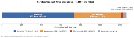
By Shantanu Patankar, and Azin Heidarshenas As part of Azure's MLPerf Training v6.0 submission, we scaled Llama 3.1 405B (NVFP4) pretraining to 8,192 GB200 GPUs across 128 racks on Azure's Fairwater infrastructure, converging in 7.07 minutes (MLPerf Training Blog). Llama 3.1, with 405 billion active parameters, has the highest active parameter count among all models in the MLPerf suite. Getting a model of this scale to train efficiently requires a cascade of tightly coupled choices around parallelism, batch sizing, and network placement. This post shares what we learned from bringing up and scaling Llama 3.1 405b on Fairwater at frontier scale. Three insights emerged: Even at 8K+ GPU scale, Llama 3.1 405B training remains compute-bound, with Feed forward Network (FFN) kernels dominating execution Topology-aware mapping is the key enabler of 8000+ GPU scale Scaling efficiency is governed by convergence dynamics, not system or network limits The rest of this post explains how these effects appear in practice. Where Does the Time Go Inside One Iteration, and What Are the Bottlenecks? Llama 3.1 405B is a dense transformer with 126 layers, each consisting of a self-attention block (QKV projections and attention) followed by a feed-forward network (FFN). To understand what limits performance at scale, we profiled steady-state iterations and broke down where time is spent, as shown in Figure 1. A single training step (Global Batch Size=1024) takes approximately 1.27s. 1: Compute vs Communication Breakdown of Llama 3.1 405B (Global Batch Size=1024) Compute: Roughly 57% of the training iteration wall time (~733 ms) is spent in compute. GEMM kernels dominate, accounting for 74% of that compute time. What is striking is how concentrated the compute is. The FFN up-projection and down-projection GEMMs alone consume ~54% of total compute (~397 ms). Everything else, including QKV projections, attention, softmax, normalization, etc., shares the remaining 46%. the FFN clearly dominates and is the primary driver of compute time. Communication: The system operates across two communication domains: high-bandwidth NVIDIA NVLink (NVL) within a rack (scale-up, 72 GPUs) and Azure’s Multipath Reliable Connection (MRC) network across racks (scale-out). The total communication work is 853 GPU-ms. Nearly 42% of this overlaps with compute or other communication (with MRC overlapping NVL), leaving only ~500 ms on the critical path. This is the portion that directly impacts step time, as shown in Figure 1. Of this ~500 ms critical-path communication, NVLink accounts for nearly all of it, while MRC contributes just 1.6%. Intra-rack NVLink communication on the critical path accounts for 37.8% (~479 ms). This includes Tensor Parallelism (TP), Pipeline Parallelism (PP), and Context Parallelism (CP) exchanges on the 1.8 TB/s intra-rack NVLink fabric, as well as pipeline bubbles, where stages idle between micro-batches. Although substantial, in a weak scaling regime, where each rack handles a fixed shard of the workload, NVLink communication per rack remains constant as we scale. MRC communication covers gradient synchronization across all DP ranks. Although it represents a substantial amount of communication work, it overlaps heavily with both NVLink communication and compute. As a result, only 1.6% (~20 ms) remains on the critical path. The cross-rack MRC network is nearly invisible in the step profile. The workload is compute-bound even at 8192 GPU scale, with FFN as the center of gravity. Any improvement to FFN kernel efficiency (precision, tiling, scheduling) translates almost directly into faster training steps. Why Is Topology-Aware Mapping the Key Enabler of Scale? In the first section, we showed that cross-rack MRC communication accounts for just 1.6% of step time. This result comes from how parallelism is mapped to the cluster’s two-tier network. Training Llama 3.1 405B distributes work across four dimensions. Tensor Parallelism (TP), Pipeline Parallelism (PP), and Context Parallelism (CP) split the model and sequence across GPUs, communicating frequently throughout each step. Data Parallelism (DP) replicates the model and synchronizes gradients once per step. The key difference: TP, PP, and CP are latency-sensitive. DP communication can be overlapped with compute, along with other NVLink-based communication. The design principle follows directly: keep latency-sensitive dimensions on the fastest links, and push traffic that can be overlapped with compute to the scale-out fabric On Azure's Fairwater cluster, each rack provides a 72-GPU NVLink domain at 1.8 TB/s. We use 64 GPUs per rack and constrain TP × PP × CP = 64, so one complete model-parallel shard fits within a single rack. Scaling to more racks adds DP replicas, with gradient synchronization flowing across the 100 GB/s Multipath Reliable Connection (MRC) network, the traffic that hides almost entirely behind compute. We swept TP, PP, and CP at fixed DP = 8 and GBS = 1152 to isolate the effect of communication efficiency on throughput. TP4–PP8–CP2 achieves the highest TFLOPS/GPU among the feasible configurations, reaching an Model FLOPs Utilization (MFU) of 26.45% as shown in Figure 2. What Limits Scaling Efficiency at 8K+ GPU Scale? We scaled Llama 3.1 405B training from 40 to 128 racks, adjusting MiniBS (per-DP-shard batch size, i.e., Global Batch Size ÷ DP) and Global Batch Size (GBS) at each scale point to balance GPU utilization against convergence efficiency. Training time drops from 18.79 minutes to 7.07 minutes, representing 83% scaling efficiency relative to the 40-rack baseline as shown in the table below. Racks GPUs MiniBS (GBS/Racks) Global Batch Size (GBS) Time-to-Train 40 2,560 24 960 18.79 min 64 4,096 16 1024 12.86 min 112 7,168 8 896 7.75 min 128 8,192 8 1,024 7.07 min Notice that MiniBS shrinks as we scale. MiniBS determines how much work each GPU processes per step and is the primary driver of step time. As we scale by increasing DP (one replica per rack), the global batch size grows proportionally unless MiniBS is reduced. Higher MiniBS improves per-step GPU utilization, but at scale it inflates GBS, and beyond a critical batch size the model requires quadratically more samples to converge. So we trade per-step throughput for faster end-to-end convergence, reducing MiniBS from 144 at 8 racks to 8 at 128 racks. MiniBS cannot be reduced below 8 in our setup because PP = 8 requires at least one microbatch per pipeline stage to keep the pipeline fully utilized. Since MiniBS cannot drop further, adding more racks only increases GBS, pushing deeper into the convergence penalty. At large scale, the optimal configuration minimizes time-to-train, not per-step throughput. The 83% scaling efficiency gap is not a network or system bottleneck. It is inherent to the benchmark's convergence dynamics. Conclusion MLPerf Training v6.0 provides a practical lens into how frontier-scale LLM systems behave under real constraints. Azure’s Llama 3.1 405B submission, which achieved a leading result at 8K+ GPU scale, highlights how performance at this level is shaped not just by infrastructure, but by the interaction of compute, topology, and convergence. Scaling efficiently at this level requires aligning these factors with the workload, not just adding more compute. View Azure's MLPerf Training v6.0 results. Read Azure's MLPerf v6.0 announcement blog. Acknowledgement This work was made possible through strong collaboration across multiple teams. We thank Prabhat Ram for his guidance throughout this effort, along with Mark Gitau, Amirreza Rastegari, Ojasvi Bhalerao, Sai Kovouri, Adam Hough, Bhupender Thakur, Nandini Ramanathan, Manasa Govindu, Sanian Gaffar, Ekrem Aksoy, Matthew Kappel, John Rankin, Girish Bhatia, Sreevatsa Anantharamu, Scott Moe, Yang Wang, and Jithin Jose — as well as many others across Azure and NVIDIA who supported this effort.
Azure Sets a New Performance Record for LLM Training Benchmark at Extreme Scale
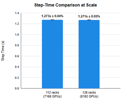
Azure achieved the most performant MLPerf Training v6.0 result to date for Llama 3.1 405B, with a time-to-train of just over seven minutes according to MLCommons. This loadbearing benchmark measures how communication overhead and system stability dominate training performance, where Azure’s full stack, end-to-end advantages shine. Azure scaled to 2,048 NVIDIA GB200 NVL72 compute tray nodes spanning 128 racks (8,192 GPUs), assembling the largest reported GB200 NVL72 cluster to date in MLPerf Training. As model sizes continue to grow into hundreds of billions of parameters, achieving this level of performance consistently requires not only massive compute capacity, but also a highly efficient communication infrastructure. To meet the demands of the massive training workloads, Azure’s Fairwater AI supercomputing infrastructure offers high-performance GPU scale-up domains with resilient, scale-out networking. Fairwater is optimized for frontier-scale distributed AI training, where communication overhead and synchronization latency can become major scaling bottlenecks at multi-thousand GPU scale. This remarkable result was possible by leveraging fifth-generation NVIDIA NVLink at 1,800 GB/s per GPU for intra-rack communication and Azure’s 100 GB/s MRC (Multipath Reliable Connection) fabric accelerated by NVIDIA DOCA and connected with NVIDIA ConnectX-8 and NVIDIA Spectrum-X Ethernet switches for inter-rack communication. What Enabled Scaling Llama 405B to 8,192 GPUs on Azure Achieving efficient training at this scale requires more than raw compute. Three architectural ingredients came together to make this result possible: High operational efficiency of NVLink scale-up domains, providing fast intra-rack GPU-to-GPU communication. Resiliency and stability of Azure’s MRC scale-out networking fabric, built on NVIDIA ConnectX-8 SuperNICs and Spectrum-X Ethernet switches, delivering 100 GB/s per GPU across racks. Topology-aware workload mapping, aligning parallelism strategies with the underlying network structure. Large-scale LLM training is fundamentally synchronous. At every training step, GPUs perform forward and backward passes followed by gradient synchronization across ranks. Because all GPUs must stay in sync, training progress is ultimately limited by the slowest rank — any time spent waiting on the network directly increases overall step time. For the Llama 405B benchmark, the workload is distributed across four dimensions of parallelism: Tensor, Context, Pipeline, and Data parallelism. Each generates different communication patterns, with some communication sitting directly on the critical training path. If left unmanaged, communication overhead can quickly become a major bottleneck at scale. The key insight is that not all communication is equally latency-sensitive. Some communication must be completed before computation can continue, while other communication can overlap with compute. Tensor-Parallel and Context-Parallel communication sit directly on the critical compute path, meaning each layer must wait for its collective operation to complete before execution can proceed. Pipeline-Parallel communication is also on the critical path, but across stages rather than within a layer (i.e., the next stage cannot begin processing its data until the previous stage has transferred its gradients). To minimize latency, all three are placed on the high-bandwidth NVLink domain, which provides up to 1,800 GB/s per GPU. Data-Parallel communication, on the other hand, can overlap with backward compute because gradient reduction runs alongside the backward pass and does not immediately block the next operation. This traffic is carried over the MRC scale-out network. The impact of such mapping is clear at scale. Our profiling shows that cross-rack MRC communication contributes just ~20 ms of exposed time on the critical path of a ~1.27 s training step (≈1.6% of step time). This communication — primarily gradient synchronization across all ranks — is well overlapped by compute and NVLink traffic, making the scale-out network nearly invisible to training performance. Stable Step Time as the Cluster Grows To evaluate execution stability as the cluster scales, we compared our GB200 NVL72 128-rack submission against a 112-rack configuration used for this experiment. In the Llama 405B workload, the critical path of each training step is dominated by compute (forward and backward GEMMs) together with latency-sensitive Tensor-Parallel and Context-Parallel communication over NVLink. Importantly, neither of these changes as the cluster scales out. Cross-node communication, such as Data-Parallel collectives and Pipeline-Parallel transfers over the MRC network, runs concurrently with backward compute and remains largely hidden behind computation. This overlap is sustained only if cross-node communication remains fast and predictable. Any network instability, congestion, or synchronization jitter would reduce this overlap and expose communication on the critical path, directly increasing overall step time. Figure 1. Step-time vs cluster size at scale This is exactly what we observe in practice under a weak scaling model, where we maintain a constant workload per GPU while scaling total cluster capacity. As shown in Figure 1, step time remains nearly identical at scale, measuring 1.2734 seconds at 112 GB200 NVL72 racks (7,168 GPUs) and 1.2712 seconds at 128 racks (8,192 GPUs) — a difference of just 2 ms. This corresponds to a near-perfect 99.8% weak scaling efficiency as we expanded the cluster by an additional 1,024 GPUs. Step-time variance also remains extremely low (±0.04–0.05%), confirming stable and predictable execution at extreme scale. This directly translates to maximized hardware utilization and an accelerated overall time-to-train, demonstrating the resiliency of Azure’s MRC scale-out network. Acknowledgement This work was made possible through strong collaboration across multiple teams. We would like to especially recognize Shantanu Patankar for his contributions to execution and performance analysis and Mark Gitau for his contributions to data preparation and experiment support as core contributors, and extend our thanks to Amirreza Rastegari, Ojasvi Bhalerao, Sai Kovouri, Adam Hough, Nandini Ramanathan, Manasa Govindu, Sanian Gaffar, Ekrem Aksoy, Bhupender Thakur, Matthew Kappel, John Rankin, Girish Bhatia, Sreevatsa Anantharamu, Scott Moe, Yang Wang, and Jithin Jose, as well as many others across Azure and NVIDIA who supported this effort.
Training 100B+ Models on a Single GPU: What MegaTrain Changes - and What It Means for Azure
The Paradigm Shift in Model Training The conventional wisdom in deep learning has been simple: bigger models require bigger infrastructure. Training a 100-billion parameter language model traditionally demands massive GPU clusters with terabytes of combined memory, where each GPU holds portions of the model simultaneously. This assumption has shaped the entire AI infrastructure landscape, driving demand for high-memory accelerators and complex distributed training frameworks. A new paper named MegaTrain (Yuan et al) by research teams at NotreDame and Lehigh universities, changes this paradigm by demonstrating that model size need not be limited by GPU memory capacity. Instead of treating memory as a container that must hold the entire model, MegaTrain treats it as a cache through which model components flow during computation. This architectural inversion enables training models orders of magnitude larger than available GPU memory, transforming what was thought to be a hardware limitation into a software scheduling problem. The implications extend beyond academic curiosity to practical infrastructure decisions, particularly for cloud platforms like Azure where GPU configurations, interconnect topologies, and cost structures create distinct optimization landscapes. The Memory Bottleneck in Traditional LLM Training Large language model training faces a fundamental memory constraint that grows with model scale. A typical 100-billion parameter model with mixed-precision training may require in excess of 1 Terabyte of memory when taking into account weights and optimizer states. Activation memory adds another substantial overhead, particularly for long sequences where intermediate layer outputs must be retained for backpropagation. Traditional training approaches keep all parameters, gradients, and optimizer states resident in GPU memory simultaneously, creating a hard ceiling on trainable model size. Standard datacenter GPUs like the NVIDIA A100 with 80GB memory can barely accommodate models beyond 20 billion parameters with reasonable batch sizes, while consumer-grade GPUs with 16-24GB memory are restricted to models under 5 billion parameters. This memory wall has forced the AI community toward distributed training strategies like pipeline parallelism, tensor parallelism, and data parallelism, each adding communication overhead, synchronization complexity, and infrastructure costs. The memory bottleneck becomes particularly acute during gradient accumulation and optimizer updates, where transient memory peaks can trigger out-of-memory errors even when average utilization suggests sufficient capacity. The Key Insight: Inverting the Memory Hierarchy MegaTrain's core innovation inverts the traditional memory hierarchy by treating GPU memory as a streaming cache rather than a static container. In conventional training, the model resides in GPU memory while slower storage sits idle except for checkpoint loading. MegaTrain reverses this relationship: the full model lives in high-bandwidth storage like NVMe SSDs, with only the actively computing layer residing in GPU memory at any moment. This architectural inversion exploits the sequential nature of neural network computation: forward and backward passes process layers in deterministic order, creating predictable access patterns amenable to prefetching and streaming. The approach transforms the memory constraint from a capacity problem into a bandwidth problem where success depends on streaming layers between storage and GPU fast enough to keep compute units saturated. Modern NVMe SSDs provide 7-14 GB/s sequential read bandwidth, while PCIe 4.0 x16 offers 32 GB/s bidirectional throughput, creating sufficient headroom for layer streaming when properly pipelined. This memory hierarchy is the basis for a fundamental architectural shift, through which MegaTrain moves from memory-bound scaling to bandwidth-bound scaling. MegaTrain Architecture and Core Mechanisms MegaTrain implements memory hierarchy inversion through four interlocking mechanisms that together enable efficient single-GPU training of massive models. The architecture maintains model parameters, optimizer states, and gradients in host memory or NVMe storage, streaming only the actively computing layer into GPU memory. Each training iteration processes layers sequentially: during the forward pass, layers stream from storage to GPU, compute activations, then stream back to make room for the next layer. The backward pass reverses this flow, streaming layers in reverse order to compute gradients. Critically, MegaTrain maintains minimal GPU memory footprint by immediately evicting each layer after computation rather than accumulating them. The system achieves this through careful orchestration of four core techniques that transform naive layer streaming from a theoretical possibility into a practical training method. Layer-wise streaming provides the foundation by decomposing model computation into independent sequential operations. Pipelined execution overlaps data movement with computation to hide transfer latency. Block-wise recomputation trades redundant forward passes for reduced activation memory. Stateless execution eliminates persistent GPU state to maximize available memory for active computation. Together, these techniques enable training throughput within 2-5x of conventional in-memory training while supporting models 10-100x larger than GPU memory capacity. Let’s look at each of these techniques in detail. Layer-Wise Streaming: Sequential Model Decomposition Layer-wise streaming exploits the inherently sequential structure of neural network computation to decompose model execution into memory-independent stages. Each transformer layer performs a self-contained computation: it receives input activations, applies attention and feedforward transformations, and produces output activations for the next layer. MegaTrain leverages this modularity by loading exactly one layer's parameters into GPU memory, computing its forward pass, storing the output activations, then immediately evicting the layer to make room for the next. During backpropagation, the process reverses: layers stream in reverse order, recompute their forward pass from stored input activations, compute gradients, and stream back to storage. This approach reduces peak GPU memory from the sum of all layer parameters to the size of the single largest layer plus activation storage. For a 100-billion parameter model with 80 transformer layers, each layer contains approximately 1.25 billion parameters requiring 2.5GB in FP16, compared to 200GB for the full model. The memory savings enable training on GPUs that would otherwise be incapable of holding even a fraction of the model. Layer-wise streaming does introduce computational overhead: each layer must be loaded and evicted during both forward and backward passes, creating 4x the parameter transfer volume compared to conventional training. However, modern interconnect bandwidth and careful prefetching largely mitigate this overhead when properly pipelined. Pipelined Execution: Overlapping Transfer and Compute Pipelined execution hides layer streaming latency by overlapping data transfers with GPU computation, ensuring compute units remain saturated despite continuous parameter movement. MegaTrain maintains a three-stage pipeline: while the GPU computes layer N, the system prefetches layer N+1 from storage to host memory and simultaneously evicts layer N-1 back to storage. This overlapping execution exploits the independence of CPU-GPU data transfers and GPU computation in modern architectures. PCIe transfers and GPU kernels execute concurrently when properly scheduled using asynchronous CUDA streams, allowing near-complete latency hiding if transfer time does not exceed computation time. For typical transformer layers, forward pass computation takes 50-200ms depending on batch size and sequence length, while transferring a 2.5GB layer over PCIe 4.0 x16 at 16 GB/s requires only 156ms, fitting comfortably within the computation window. The pipeline achieves optimal efficiency when transfer bandwidth and computation throughput are balanced, creating a predictable performance model based on layer size, batch configuration, and interconnect speed. The three-stage pipeline pattern - prefetch, compute, and eviction - interleaves to maintain continuous GPU utilization, as illustrated in the diagram above. Block-Wise Recomputation Block-wise recomputation addresses the activation memory bottleneck by trading computation for memory through selective forward pass recalculation. In standard training, all intermediate activations from the forward pass must be retained for gradient computation during backpropagation, consuming memory proportional to model depth and batch size. MegaTrain instead stores only a subset of checkpoint activations at regular intervals, recomputing intermediate values on-demand during the backward pass. For a model with 80 layers, storing checkpoints every 10 layers reduces activation memory by 90 percent at the cost of recomputing 9 out of 10 layers during backpropagation. This trade-off proves favorable because forward pass computation is relatively cheap compared to the memory savings, and recomputation can be pipelined with layer streaming. Stateless Execution Stateless execution complements recomputation by eliminating all persistent GPU state between layer computations. After processing each layer, MegaTrain immediately evicts not only parameters but also optimizer states like momentum buffers and variance estimates, keeping only the minimal activations needed for gradient flow. This aggressive state eviction maximizes available GPU memory for the active layer's computation, enabling larger batch sizes and longer sequences within fixed memory budgets. Together, block-wise recomputation and stateless execution transform MegaTrain's memory footprint from O(model_size) to O(largest_layer + checkpoint_activations), typically reducing requirements by 50-100x for models in the 100-billion parameter range. W- Weight prefetch, F/R/B – Computation, G – Gradient offload Source: Yuan, Zhengqing, et al. MegaTrain: Full Precision Training of 100B+ Parameter Large Language Models on a Single GPU Performance Results and Achievements MegaTrain demonstrates practical viability by training models far exceeding GPU memory capacity with acceptable performance overhead. The paper reports an implementation that successfully trained a 175-billion parameter model on a single NVIDIA A100 GPU with 80GB memory. Using conventional techniques, that same hardware configuration would support only 15-20 billion parameters. When using this conventional configuration as the baseline to compare to, MegaTrain throughput reached 45 percent of the baseline in-memory training speed, translating to approximately 2.2x wallclock time for equivalent training steps. For smaller models at 30-billion parameters, throughput exceeded 65 percent of baseline as the ratio of computation to transfer improved. The chart demonstrates the inverse relationship between model size and throughput efficiency. As model parameters increase from 30 billion to 175 billion, throughput degrades linearly from 65% to 45% of baseline, validating the predictable performance characteristics of the streaming approach. This degradation reflects the increasing ratio of layer count to computation time as models grow larger. Memory efficiency gains are substantial: peak GPU memory utilization remained under 40GB throughout training regardless of model size, with the remainder allocated to batch size expansion that partially offset streaming overhead. The system sustained 12-14 GB/s effective storage bandwidth during training, approaching theoretical NVMe limits and validating the pipelined streaming approach. The memory utilization chart reveals MegaTrain's fundamental breakthrough: GPU memory consumption remains nearly constant across vastly different model sizes. While conventional training would require proportionally more GPU memory as models grow, MegaTrain keeps peak utilization between 35GB and 40GB regardless of whether the model has 30 billion or 175 billion parameters. This flat memory profile enables single-GPU training of models that would otherwise require expensive multi-GPU configurations. Scaling analysis revealed predictable performance characteristics: throughput degraded linearly with model size as layer count increased, while improving with batch size as computation became more dominant relative to fixed transfer costs. Energy efficiency comparisons showed single-GPU MegaTrain consuming 85 percent less power than equivalent 8-GPU distributed training for the same model, though at 2.2x longer duration resulting in 40 percent total energy savings. Running MegaTrain on Azure NC-Series GPUs Azure's NC-series GPU virtual machines provide diverse configurations for MegaTrain deployment, each with distinct performance characteristics shaped by GPU type, interconnect topology, and storage options. The NC A100 v4 series offers NVIDIA A100 GPUs with 80GB memory over PCIe 4.0 interfaces, directly matching the original MegaTrain research configuration. These instances provide 32 GB/s bidirectional PCIe bandwidth sufficient for layer streaming without bottlenecking on parameter transfers for models up to 200-billion parameters. Storage configuration critically impacts MegaTrain performance: Azure Premium SSD v2 delivers up to 16 GB/s throughput with appropriate provisioning, while local NVMe SSDs on storage-optimized instances can reach 7-14 GB/s depending on VM size. The NC series of VMs provides a large amount of system memory, local NVMe storage and GPUs, creating an ideal environment for MegaTrain's host memory and storage requirements. Importantly, Azure's NC-series instances use PCIe-connected GPUs rather than NVLink-connected configurations, making interconnect bandwidth the primary performance constraint rather than GPU compute capacity. Cost analysis favors MegaTrain for experimentation and medium-scale training: a single NC A100 v4 instance costs ~4 dollars per hour compared ~30 dollars per hour for an 8-GPU NDv4 instance, enabling 8x cost reduction for workloads tolerant of 2-3x longer training duration. Code for MegaTrain is available on the project’s Github repository at https://github.com/DLYuanGod/MegaTrain. Supported models at the time of writing include Qwen 2/2.5/3/3.5/3.5 MoE, Llama 2/3/3.1/3.2/3.3/4, Mistral, Mixtral, DeepSeek Code/R1, Phi-3/4, Gemma 2/3, as well as some others. Critical Constraint: PCIe Bandwidth vs NVLink The interconnect bandwidth hierarchy creates fundamentally different performance envelopes for MegaTrain on Azure compared to specialized research hardware. PCIe 4.0 x16 connections on Azure NC-series instances provide 32 GB/s bidirectional bandwidth between CPU and GPU. For MegaTrain's layer streaming workload, CPU-GPU bandwidth matters most since model parameters flow from host memory or NVMe storage through PCIe to GPU memory. PCIe 4.0's 32 GB/s bidirectional capacity proves sufficient for models up to 200-billion parameters when combined with aggressive prefetching and eviction pipelining but becomes a hard bottleneck for larger models where layer transfer time exceeds computation time. Trade-Offs and Limitations MegaTrain introduces several trade-offs that practitioners must evaluate against infrastructure constraints and training objectives. Training throughput degrades to 40-65 percent of baseline depending on model size, extending wallclock training time by 1.5-2.5x for equivalent iteration counts. This slowdown proves acceptable for research experimentation and low-frequency retraining but may be prohibitive for production pipelines requiring rapid iteration. Memory efficiency gains come at the cost of increased storage I/O: a full training run generates 4x the parameter transfer volume compared to conventional training due to bidirectional streaming during forward and backward passes. This I/O amplification accelerates SSD wear and may impact cost for cloud storage with throughput-based pricing. Implications for AI Infrastructure and Azure Strategy MegaTrain's viability reshapes infrastructure planning assumptions for AI training workloads, particularly in cost-constrained environments where model size exceeds available GPU memory. Organizations can defer expensive hardware upgrades by exploiting existing GPU capacity more fully through memory hierarchy inversion, extending the useful life of current hardware generations. Cloud platforms like Azure benefit from increased flexibility in instance sizing: users can select GPU types based on compute requirements rather than being forced into high-memory configurations solely for capacity. This decoupling enables better price-performance optimization by matching compute intensity to GPU type while relying on storage for capacity scaling. The approach particularly suits Azure's NC-series positioning as a cost-effective alternative to specialized AI instances, turning PCIe bandwidth into an acceptable constraint rather than a disqualifying limitation. Research teams gain the ability to prototype and validate large model architectures without provisioning expensive multi-GPU clusters, accelerating iteration during early development phases. However, production deployment strategies should carefully evaluate MegaTrain's throughput trade-offs against distributed training alternatives: the 2-3x slowdown may be unacceptable for latency-sensitive pipelines despite cost savings. Infrastructure teams should prioritize NVMe storage provisioning and PCIe 4.0/5.0 support (for example, by using newer GPU types such as the H100) when deploying MegaTrain-compatible environments, as storage bandwidth directly determines achievable performance. Long-term, the techniques validate a broader trend toward memory-disaggregated computing where storage, memory, and compute scale independently rather than in fixed ratios determined by hardware packages.AI Infrastructure Preflight at User space: Validating Multi Node, Multi GPU Slurm Clusters
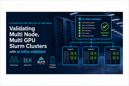
Every team that operates GPU clusters for AI has seen this pattern. The cluster boots, GPUs are visible, and scheduling works at a basic level. Then the first distributed training run stalls in NCCL initialization, fails during rank rendezvous, or silently maps ranks to the wrong devices. The issue is often not in training code. It is in infrastructure consistency across scheduler, runtime, drivers, networking, and process topology. The goal of ai-infra-validator is straightforward: Run a fast user space preflight before expensive training jobs. Validate distributed initialization for multi node, multi GPU workloads. Confirm GPU affinity and rank mapping are correct. Verify NCCL communication fabric can complete a collective ring under Slurm. This post walks through the implementation in detail, explains why each part exists, and shows how to operationalize it in real HPC AI environments. What the project validates Zero-dependency user space smoke test for AI clusters. Validates multi-node PyTorch DDP initialization, GPU affinity, and NCCL fabric connectivity under Slurm orchestration. Git Repo: ai-cluster-validator In practical terms, this checks that: Slurm launches the expected number of ranks per node. Distributed process group creation with NCCL succeeds. Each rank binds to the expected local GPU. Cross-rank all-reduce completes and converges. Node level telemetry confirms software and fabric state. This is not a performance benchmark. It is a correctness and readiness gate. Tested platform profile Component Value CycleCloud 8.8.3-3667 Slurm 25.05.5 Slurm partition hpc Scheduler VM SKU Standard_D8s_v6 Compute VM SKU Standard_ND96asr_v4 OS images microsoft-dsvm:ubuntu-hpc:2204:latest and microsoft-dsvm:ubuntu-hpc:2404:latest PyTorch 2.12.0+cu130 CUDA runtime 13.0 NCCL target 2.29.7 This profile represents a common enterprise scenario where scheduler and compute nodes have different roles, and the training fleet depends on correct multi node orchestration. Step 1: Minimal user space bootstrap The bootstrap script creates a shared Python environment at /shared/apps/pytorch_env and installs the required packages: torch torchvision torchaudio psutil This choice is intentional: No dependency on containers for first-pass validation. Single environment path visible to all compute nodes. Rapid setup and repeatability for cluster operators. Command sequence: git clone https://github.com/vinil-v/ai-cluster-validator.git cd ai-cluster-validator sudo bash bootstrap_env.sh Step 2: Slurm job defines deterministic distributed topology The Slurm script expresses a clear topology contract: nodes=2 ntasks-per-node=8 gpus-per-node=8 cpus-per-task=12 From this, world size is derived as: WORLD_SIZE = SLURM_NTASKS = 2 x 8 = 16 The script also configures network and NCCL behavior: NCCL_DEBUG=WARN NCCL_IB_DISABLE=0 NCCL_P2P_DISABLE=0 NCCL_IGNORE_CPU_AFFINITY=1 GLOO_SOCKET_IFNAME=eth0 NCCL_SOCKET_IFNAME=eth0 Important implementation detail: MASTER_ADDR is set to the first host in SLURM_JOB_NODELIST. MASTER_PORT is selected dynamically from the ephemeral range 49152-65535 and falls back to 29500 if needed. Why this matters: Reduces port collision risk when jobs run frequently. Avoids hardcoded rendezvous values that may fail in shared clusters. Launch path: srun --cpu-bind=none bash -c " source /shared/apps/pytorch_env/bin/activate; export RANK=$SLURM_PROCID; export LOCAL_RANK=$SLURM_LOCALID; python3 ddp_mesh_ping.py " The LOCAL_RANK handoff is critical for stable GPU affinity inside each node. Step 3: DDP initialization and rank to GPU affinity Inside ddp_mesh_ping.py, each process executes: Parse WORLD_SIZE, RANK, LOCAL_RANK, MASTER_ADDR, MASTER_PORT. Initialize torch.distributed with backend nccl and TCP init method. Set CUDA device using LOCAL_RANK. Core initialization path: dist.init_process_group( backend="nccl", init_method=f"tcp://{master_addr}:{master_port}", world_size=world_size, rank=rank ) torch.cuda.set_device(local_rank) This validates the minimum distributed contract required by real model training jobs. Step 4: Rich node and fabric telemetry in user space Each rank collects detailed metadata before the collective test: Node identity from Slurm and hostname. GPU model and VRAM from CUDA properties. System memory via psutil. CPU model from /proc/cpuinfo. OS and kernel versions. NVIDIA driver version from /proc/driver/nvidia/version. PyTorch, CUDA, and NCCL runtime versions. InfiniBand device state and link rate from /sys/class/infiniband. Basic GPU peer access capability via torch.cuda.can_device_access_peer. All rank payloads are gathered on rank 0 using dist.gather_object and printed as: Cluster hardware topology report. Node environment deep dive. Network interconnect and fabric status. This design gives platform teams one artifact that is both operational and diagnostic. Step 5: Functional collective validation After telemetry, each rank executes a lightweight DDP compute path: Build nn.Linear(10,10) on local GPU. Wrap with DistributedDataParallel. Perform forward, loss, backward. Run all_reduce on loss tensor. Compute global average loss. Pass condition is explicit in log output: SUCCESS: DDP Multi-Node AllReduce Ring Complete! This confirms that process group initialization and collective communication both completed successfully. What a successful run looks like Submission: sbatch ddp_smoke_test.slurm squeue Representative outcomes in the log: Total Execution Ranks: 16 Two nodes with local ranks 0 through 7 on each node GPU inventory aligned with expected A100 topology Active InfiniBand HCAs discovered per host NCCL socket interface set to eth0 Final success marker and computed convergence loss When these markers are present and coherent with expected hardware shape, the cluster is typically ready for distributed training bring-up. How to check the output file The Slurm script writes two artifacts per job: ai_infra_smoke_test_<jobid>.log ai_infra_smoke_test_<jobid>.err Use this exact workflow after submission: # 1. Submit and capture the job id sbatch ddp_smoke_test.slurm # 2. Check job state squeue -j <jobid> # 3. Read standard output log cat ai_infra_smoke_test_<jobid>.log # 4. Read standard error log cat ai_infra_smoke_test_<jobid>.err For stronger validation in automation, also check: Total Execution Ranks equals expected world size. Both nodes appear in the topology table with local ranks 0 through 7. NCCL/CUDA/PyTorch versions are present in the node environment section. Complete reference output Use the following full log as a known-good reference from a successful 2-node ND96asr_v4 run. Master Node IP/Hostname: ddpcluster-hpc-1 Dynamically Assigned Port: 53593 Total Execution Ranks: 16 =============================================================================================== HPC CLUSTER INTERACTION MONITOR =============================================================================================== --> Initializing DDP on Master Node : ddpcluster-hpc-1 --> Dynamic Coordination Port : 53593 --> Target World Cluster Size : 16 GPUs ----------------------------------------------------------------------------------------------- =============================================================================================== CLUSTER HARDWARE TOPOLOGY REPORT =============================================================================================== | Rank | Node Name | Local ID | GPU Model | VRAM | Sys Mem | CPU Cores | ----------------------------------------------------------------------------------------------- | 0 | ddpcluster-hpc-1 | 0 | NVIDIA A100-SXM4-4 | 39.5 GB | 885.8 GB | 96 Cores | | 1 | ddpcluster-hpc-1 | 1 | NVIDIA A100-SXM4-4 | 39.5 GB | 885.8 GB | 96 Cores | | 2 | ddpcluster-hpc-1 | 2 | NVIDIA A100-SXM4-4 | 39.5 GB | 885.8 GB | 96 Cores | | 3 | ddpcluster-hpc-1 | 3 | NVIDIA A100-SXM4-4 | 39.5 GB | 885.8 GB | 96 Cores | | 4 | ddpcluster-hpc-1 | 4 | NVIDIA A100-SXM4-4 | 39.5 GB | 885.8 GB | 96 Cores | | 5 | ddpcluster-hpc-1 | 5 | NVIDIA A100-SXM4-4 | 39.5 GB | 885.8 GB | 96 Cores | | 6 | ddpcluster-hpc-1 | 6 | NVIDIA A100-SXM4-4 | 39.5 GB | 885.8 GB | 96 Cores | | 7 | ddpcluster-hpc-1 | 7 | NVIDIA A100-SXM4-4 | 39.5 GB | 885.8 GB | 96 Cores | | 8 | ddpcluster-hpc-2 | 0 | NVIDIA A100-SXM4-4 | 39.5 GB | 885.8 GB | 96 Cores | | 9 | ddpcluster-hpc-2 | 1 | NVIDIA A100-SXM4-4 | 39.5 GB | 885.8 GB | 96 Cores | | 10 | ddpcluster-hpc-2 | 2 | NVIDIA A100-SXM4-4 | 39.5 GB | 885.8 GB | 96 Cores | | 11 | ddpcluster-hpc-2 | 3 | NVIDIA A100-SXM4-4 | 39.5 GB | 885.8 GB | 96 Cores | | 12 | ddpcluster-hpc-2 | 4 | NVIDIA A100-SXM4-4 | 39.5 GB | 885.8 GB | 96 Cores | | 13 | ddpcluster-hpc-2 | 5 | NVIDIA A100-SXM4-4 | 39.5 GB | 885.8 GB | 96 Cores | | 14 | ddpcluster-hpc-2 | 6 | NVIDIA A100-SXM4-4 | 39.5 GB | 885.8 GB | 96 Cores | | 15 | ddpcluster-hpc-2 | 7 | NVIDIA A100-SXM4-4 | 39.5 GB | 885.8 GB | 96 Cores | =============================================================================================== NODE ENVIRONMENT DEEP DIVE ----------------------------------------------------------------------------------------------- [ddpcluster-hpc-1] Details: --> CPU Microarchitecture : AMD EPYC 7V12 64-Core Processor --> Operating System : Ubuntu 22.04.5 LTS --> Kernel Base Version : 5.15.0-1110-azure --> Nvidia Driver Loaded : 580.126.20 --> PyTorch Environment : v2.12.0+cu130 --> CUDA Runtime Version : v13.0 --> NCCL Fabric Target : v2.29.7 --> Discovered InfiniBand HCAs: - mlx5_an0:1 (4: ACTIVE - 40 Gb/sec (4X QDR)) - mlx5_ib0:1 (4: ACTIVE - 200 Gb/sec (4X HDR)) - mlx5_ib1:1 (4: ACTIVE - 200 Gb/sec (4X HDR)) - mlx5_ib2:1 (4: ACTIVE - 200 Gb/sec (4X HDR)) - mlx5_ib3:1 (4: ACTIVE - 200 Gb/sec (4X HDR)) - mlx5_ib4:1 (4: ACTIVE - 200 Gb/sec (4X HDR)) - mlx5_ib5:1 (4: ACTIVE - 200 Gb/sec (4X HDR)) - mlx5_ib6:1 (4: ACTIVE - 200 Gb/sec (4X HDR)) - mlx5_ib7:1 (4: ACTIVE - 200 Gb/sec (4X HDR)) ----------------------------------------------------------------------------------------------- [ddpcluster-hpc-2] Details: --> CPU Microarchitecture : AMD EPYC 7V12 64-Core Processor --> Operating System : Ubuntu 22.04.5 LTS --> Kernel Base Version : 5.15.0-1110-azure --> Nvidia Driver Loaded : 580.126.20 --> PyTorch Environment : v2.12.0+cu130 --> CUDA Runtime Version : v13.0 --> NCCL Fabric Target : v2.29.7 --> Discovered InfiniBand HCAs: - mlx5_an0:1 (4: ACTIVE - 40 Gb/sec (4X QDR)) - mlx5_ib0:1 (4: ACTIVE - 200 Gb/sec (4X HDR)) - mlx5_ib1:1 (4: ACTIVE - 200 Gb/sec (4X HDR)) - mlx5_ib2:1 (4: ACTIVE - 200 Gb/sec (4X HDR)) - mlx5_ib3:1 (4: ACTIVE - 200 Gb/sec (4X HDR)) - mlx5_ib4:1 (4: ACTIVE - 200 Gb/sec (4X HDR)) - mlx5_ib5:1 (4: ACTIVE - 200 Gb/sec (4X HDR)) - mlx5_ib6:1 (4: ACTIVE - 200 Gb/sec (4X HDR)) - mlx5_ib7:1 (4: ACTIVE - 200 Gb/sec (4X HDR)) ----------------------------------------------------------------------------------------------- NETWORK INTERCONNECT & FABRIC STATUS ----------------------------------------------------------------------------------------------- --> Target Communication Interface (NCCL_SOCKET_IFNAME) : eth0 --> Active Telemetry Tracking Level (NCCL_DEBUG) : WARN --> Inter-GPU Topo Link Verification : Active (P2P/NVLink Capable) ----------------------------------------------------------------------------------------------- SUCCESS: DDP Multi-Node AllReduce Ring Complete! --> Computed System Verification Convergence Loss : 1.398719 =============================================================================================== Why this is effective for platform operations For AI infrastructure teams, this pattern is highly effective because it is: Fast: can be run after every change window. Deterministic: same topology contracts every run. Actionable: output includes enough context for first-level triage. Low friction: user space only, no heavy control plane dependencies. This supports common operating workflows: Day-0 cluster acceptance. Day-1 patch validation after driver, kernel, or image changes. Regression gate in golden image pipelines. Preflight before large multi node model training jobs. Practical guidance for extending to larger clusters Adjust Slurm directives for nodes and tasks per node. Keep one rank per GPU unless validating alternate placement policy. Set NCCL_SOCKET_IFNAME and GLOO_SOCKET_IFNAME according to your network policy. Preserve the dynamic MASTER_PORT logic to avoid static collisions. Keep the success marker string stable so automation can parse it. Closing perspective Most distributed training failures are expensive because they are discovered late. A user space preflight that validates scheduler topology, rank rendezvous, GPU affinity, and NCCL collectives provides a high value guardrail before production starts. ai-infra-validator is a practical implementation of that guardrail. It is compact, transparent, and aligned with how real Slurm based AI clusters operate. For teams running multi node multi gpu training at scale, this kind of preflight should be a standard operational gate.Building resilient networks for AI supercomputers
By Valerie Cutts and Jithin Jose Last fall we introduced Fairwater, the world’s most powerful AI datacenter. Delivering a system of this scale required rethinking how Azure designs supercomputers, especially the scale-out network. Today, we are sharing more about the networking innovations that have made Fairwater possible. In this post, we share what’s unique about networking at extreme GPU scale and the system-level design choices required to enable large synchronous training jobs to run reliably, even during network failures. We are also publishing, in partnership with others, the open-source Multipath Reliable Connection (MRC) specification and software interfaces, and open-sourcing the associated libraries. Fault-tolerant scale-out networking At extreme scale, synchronous training amplifies the impact of routine network faults, turning packet drops, slow links, and partial failures into stalls, restarts, and wasted GPU time. As we describe in our MRC paper, the path forward is to treat failure as normal and design the network as an integrated system that: Scales to 100K+ GPUs using a two level, multi-path topology to enable enough redundancy Balances load evenly across the fabric to prevent congestion Recovers predictably and gracefully during failures Uses less power than three- or four-layer single-plane topologies As outlined in the Multipath Reliable Connection Specification, Microsoft partnered with AMD, Broadcom, Intel, NVIDIA and OpenAI to jointly address this problem, focusing on changes to transport and network design needed to support training at extreme scale. Instead of relying on lossless fabrics and dynamic routing, we collectively designed, built, and deployed Multipath Reliable Connection (MRC), which draws upon lessons from the Ultra Ethernet Consortium (UEC), and paired it with a multiplane network topology, enabling reliable training jobs even when links, switches, or paths fail. The endpoint–driven transport created a simpler, more resilient network that delivers: More resilient, predictable training at very large scale Large training jobs continue making steady forward progress despite routine network faults, reducing stalls and restarts and improving time-to-train as cluster size increases. Better utilization of expensive GPU infrastructure By avoiding tail latency amplification and repeated recovery cycles, GPUs spend more time doing useful work instead of waiting on synchronization or replaying lost computation, improving overall efficiency and cost effectiveness. Automatic adaptation at machine timescales Failure detection, load balancing, and recovery happen fast enough to keep up with the rate and complexity of faults in 100K+ GPU systems, well beyond what manual intervention or control-plane convergence can achieve, allowing the system to remain stable as scale increases. In the Fairwater supercomputer, enabling graceful degradation in the scale-out network improves training throughput versus traditional transports and architectures. In combination with a multi-plane topology design, MRC increases the time that installed NVIDIA GPUs perform useful computation. A shift in philosophy: End-to-end control The central design decision behind MRC is to shift responsibility for load balancing and failure handling from complex network switch control planes to the network endpoints with end-to-end controls. The network endpoint controls the path selection and can optimally use a set of paths based on feedback from the network. MRC extends the RoCE Reliable Connection (RC) transport to support true multipath operation. Instead of binding a queue pair to a single path, MRC sprays packets across many paths simultaneously, making performance far less sensitive to any single slow or failed link. Several design elements are critical to enable end-to-end control. Every packet carries enough information for the receiver to place it directly into memory, even if packets arrive out of order. Selective acknowledgments enable rapid retransmission of only the packets that were lost. Packet trimming signals network congestion swiftly without forcing full packet drops, enabling efficient congestion control. MRC disables Priority Flow Control (PFC) entirely and runs Ethernet in best-effort mode, avoiding global pauses that can devastate tail latency or lead to fabric-wide deadlock behavior. The system enables seamless self-recovery from network hardware failures. The result is a transport protocol that expects loss, adapts quickly, and continues making progress even when parts of the fabric misbehave. Rethinking topology: Multi‑plane design Transport alone is not enough. To complement MRC, we implemented a two-tier, multiplane network topology in Fairwater using high-radix switches. Our network design splits each NIC into multiple lower speed ports (i.e. eight x 100 Gbps) and builds multiple parallel network planes. This multi-plane design enables a more compact topology, as opposed to a traditional three-tier Clos Network running at 800 Gbps/port. Our 2-layer multi-plane topology design offers several advantages: Enables connecting 100K+ GPUs with just two tiers of network. Lower latency since packets traverse fewer switches. Reduced impact of network issues on overall job completion, while we see single switches connected to more servers, the individual impact is reduced by spreading the failure, decreasing the performance impact to the overall job. Reduced hardware and power costs compared to designs with additional network layer, without compromising on GPU scale. Most importantly, the network becomes more tolerant of partial failures, so jobs continue with slightly reduced bandwidth rather than failing outright. Multiplane networks work efficiently only when traffic is evenly distributed across all planes and paths. This is where MRC’s packet spraying and path aware congestion response is essential. Figure 1: Example of two-tier multi-plane topology using 512 x 100 GbE switches: 512 T0s x 256 NICs = 131,072 NICs Static SRv6: Fewer moving parts, more predictability In many data center networks, switches rely on Border Gateway Protocol (BGP) or other dynamic routing protocols. We removed dynamic routing from our design; instead, packets are source-routed using IPv6 Segment Routing (SRv6). Each packet encodes the end-to-end network path using compact microsegment IDs (uSIDs). At first glance, static routing seems counterintuitive in failure-prone environments. At extreme scale, however, dynamic routing is more of a liability than an asset. Namely, if two or more switches try to reroute packets at the same time, network behavior becomes unpredictable and harder to diagnose. Interactions between adaptive routing and adaptive transport can be hard to resolve and harder to debug at larger scale. MRC, on the other hand, handles path health and rapid failover at the transport layer. When static routing is used, it enables precise health feedback for each of the different network paths from that network endpoint. Because probe (test) packets follow the same paths as data packets, operators gain accurate, ground-truth insight into fabric health without depending on switch control planes, which are themselves a common source of failures. Additionally, SRv6 routing allows network operators to utilize out-of-band monitoring frameworks to accurately identify link failures and device faults, which has been particularly valuable in managing large-scale AI clusters. Static SRv6 ensures paths are deterministic, making problems easier to reproduce, debug and, ultimately, more stable over time. Failure as a normal operating condition In production, failures are expected by design—link flaps, partial failures, and even switch reboots are routine at this scale. With MRC, many of these events no longer impact training workloads. Repair actions proceed in parallel, while MRC dynamically routes around failed paths. As repairs complete, MRC discovers and validates the restored paths before seamlessly reintegrating them—entirely transparent to the training application. In summary: Systems degrade gracefully Losing a NIC port reduces available bandwidth proportional to the lost port but does not crash jobs Flapping T0–T1 links often go unnoticed by applications Switches can be rebooted without coordinated drain or rerouting of the system For massive scale training runs, this translates into higher effective uptime, fewer interrupted jobs, and more training throughput. Figure 2: Bidirectional-bandwidth measurements with pt-pt RDMA Perftest while a T0 switch was taken down. Results indicate that the overall bandwidth dropped in proportion to the T0 switch bandwidth, but without failing the job Figure 3: Bidirectional-bandwidth measurements with RDMA Perftest while T1 switch is failed and restored. Results indicate that no impact in performance as MRC was able to route around the bad switch Measured results at scale This is not just a thought exercise: Microsoft and OpenAI have both run extensive experiments and record-scale training jobs, showing only brief, bounded performance dips during significant network faults, followed by rapid recovery. Microbenchmarks demonstrate near line-rate bandwidth and predictable latency, even under injected loss. OpenAI describes their scale results in a recent blog post, consistent with what we observe. Taken together, multi-plane MRC with SRv6 delivers better load balancing with fewer queue pairs and substantially higher resilience to packet loss, enabling millions of networking links to connect hundreds of thousands of GPUs. Figure 4: NCCL Send-Recv Benchmark Results with 42,020 GPUs each with 800 Gbps MRC NIC showing up to 92% of theoretical peak bandwidth for large message sizes What this enables Taken together, MRC, multiplane topologies, and static SRv6 form a coherent strategy for building AI supercomputer scale-out networks that keep large synchronous training jobs moving forward under real-world fault conditions. Instead of treating loss, link flaps and partial failures as events that trigger stalls or restarts, the system is designed to fail gracefully and reach 100K+ GPUs scale at high utilization. This design approach has been deployed in Fairwater and elsewhere to train state-of-the-art models, where the result is more predictable performance for large jobs with higher effective GPU utilization. The core takeaway is simple: by assuming failures will happen and, designing for them explicitly, events that would otherwise be catastrophic become minor, manageable perturbations. Join us in advancing resilient AI infrastructure To help the broader ecosystem adopt these capabilities, Microsoft is joining key partners in releasing the MRC specification to the Open Compute Project and open sourcing key components: libMRC: MRC transport APIs NCCL MRC plugin: enables NCCL to run over MRC transport MRC shim library: enables compatible verbs applications to run over MRC with no code changes MSCCL++ with MRC support: MSCCL++ library with MRC support SONiC SRv6: enhance SRv6 with open NOS for high performance AI Ethernet We encourage others to review these contributions to the public, share feedback, and ultimately adopt these capabilities within the broader ecosystem of AI networking products, infrastructures, and workloads. Acknowledgements Advancing AI at this scale requires collaboration across the industry. At Microsoft, we value our partnerships with AMD, Broadcom, Intel, NVIDIA, and OpenAI, and our shared commitment to continuing to evolve MRC alongside the broader community. References: MRC paper: Resilient AI Supercomputer Networking using MRC and SRv6 Multipath Reliable Connection Specification OpenAI MRC blog AMD MRC blog Broadcom MRC blog NVIDIA MRC Blog libMRC APIs microsoft/mrc-verbs-shim-lib: shim library to translate ibverbs to libmrc interfaces microsoft/mrc-nccl-plugin: MRC plugin for NCCL microsoft/mscclpp: MSCCL++: A GPU-driven communication stack for scalable AI applications (with MRC support)