This is the second post in a series of posts detailing the capabilities of OLAP cubes in the Data Warehouse, a new feature that enables self-service reporting functionality added in SCSM 2012.
Architecture Overview
In the figure below, a snapshot from SQL Server Business Intelligence Development Studio (BIDS) depicts the main components that are required for OLAP cubes. These components are the Data Source, Data Source View, Cubes, and Dimensions.

Figure: View of Analysis Services's DWANalysisData DB from BIDS
Data Source:
A data source is the origin of all the data that is contained within an OLAP cube. An OLAP cube will connect to a data source to read and process the raw data to perform aggregations and calculations for its associated measures. The data source for all SCSM cubes will be the SCSM Data Marts, which includes the data marts for both Operations Manager and Configuration Manager. Authentication information about the data source must be stored in Analysis Services to establish the correct level of permissions.
Data Source View:
The data source view (DSV) is a collection of views representing the dimension, fact, and outrigger tables from the data source (i.e. the SCSM data marts). The DSV will contain all the relationships between tables such as primary and foreign keys. In other words, the DSV will specify how the Analysis Services DB will map to the relational schema and provide a layer of abstraction on top of the relational database. Using this layer of abstraction, relationships can be defined between fact and dimension tables even if none exist within the source relational database. Named calculations ,custom measures, and new attributes may also be defined in the DSV that may not natively exist in the DW dimensional schema. For example, a named calculation that defines a Boolean value for “Incidents Resolved” will calculate the value as true if an incident’s status is resolved or closed. Using the named calculation, we can now define a measure to display useful information such as the percentage of incidents resolved, the total number of incidents resolved, and the total number of incidents that are not resolved.
Another quick example of a named calculation is “ReleasesImplementedOnSchedule” which provides a quick health status check on the number of release records in which the actual end date was less than or equal to the scheduled end date.
Cubes:
A definition of OLAP cubes is given in the OLAP Cube introduction section above.
Dimensions:
A dimension in Analysis Services references a dimension from the SCSM DW. In SCSM, a dimension is roughly analogous to a ManagementPackClass. Each MP Class has a list of properties, while each dimension contains a list of attributes, with each attribute mapping to one property in a class. Dimensions allow the filtering, grouping, and labeling of data. For example, you can filter computers by the installed OS and group people into categories by gender or age. The data can then be presented in a format where the data is broken down naturally into these hierarches and categories to allow a more in-depth analysis. Dimensions may also contain have natural hierarches to allow users to “drill down” to more granular levels of detail. For instance, the Date dimension will have a hierarchy of Year → Quarter → Month → Week → Day.
In the figure below, an illustration is given of a cube that contains the Date, Region, and Product Dimension:
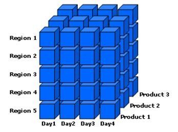
Figure: Cube with Date, Region, and Product Dimensions
Microsoft may want, for example, a quick and high level summary of the sales of the Xbox 360 gaming console in 2010. They can further drill down to get sales figures for a more focused timeframe. Business analysts may wish to examine how the sales of Xbox 360 consoles were affected by the launch of the new console design and the Kinect controller-free gaming experience. This will help them determine what sales trends are occurring and what potential revisions of business strategy are needed. By filtering on the date dimension, this information can be quickly delivered and consumed. This slicing and dicing of data is only enabled because the dimensions have been designed with attributes and data that can easily be filtered and grouped by the customer.
In SCSM 2012, all cubes will share a common set of dimensions. All dimensions will use the primary DW data mart as their source, even in multi-mart scenarios. In multi-mart scenarios, this can possibly lead to dimension key errors while processing the cube. Please refer to the troubleshooting section below on processing for more details on how to resolve this issue.
Anatomy of a Cube
This section will define the elements that define the actual cube object in Analysis Services:
Measure Group
A measure group is the exact same concept as a fact in DW terminology. Just as facts contain numeric measures in a DW, a measure group contains measures for a cube. All the measures in a cube that derive from a single fact table in a data source view also can be considered a measure group. There can be instances, however, where there will be multiple fact tables from which the measures in a cube derive from. Measures of the same granularity are united in one measure group. Measure groups define what data will be loaded into the system, how the data is loaded, and how the data is bound to the multidimensional cube.
Each measure group also contains a list of partitions, which hold the actual data in separate non-overlapping sections. Measure groups also contain Aggregation Design, which define the pre-summarized data sets that are calculated for each measure groups to improve the performance of user queries.
Measures
Measures are the numeric values users want to slice, dice, aggregate, and analyze; they are one of the fundamental reasons why users would want to build cubes on top of a data warehousing infrastructure. By using Analysis Services, users can build cubes that will apply business rules and calculations to format and display measures in a customizable format. Much of cube development time is spent on which measures will be displayed and how they will be calculated.
Measures are values that usually map to numeric columns in a DW fact table, but can also be created on dimension and degenerate dimension attributes. These measures are the most important values of a cube that are analyzed and the primary interest to end users who browse the cube. A current example of a measure that exists in our DW is ActivityTotalTimeMeasure. ActivityTotalTimeMeasure is a measure from ActivityStatusDurationFact that represents the time that each activity is in a certain status. The granularity of a measure is made up of all the dimensions that are referenced. For example, the granularity of the Relationship Fact “ComputerHostsOperatingSystem” would consist of the Computer and Operating System dimensions.
Aggregation functions are calculated on measures to enable further data analysis. The most common aggregation function is Sum. A common cube query, for example, would be to sum up the total time for all activities that are “In Progress”. Other common aggregation functions include Min, Max, and Count.
Once the raw data has been processed in a cube, users can perform more complex calculations and queries using Multidimensional Expressions (MDX) to define their own measure expressions or calculated members. MDX is the industry standard to query and access data stored in OLAP systems because SQL was not designed to work with the data model supported by multidimensional databases.
Drilldown
When a user drills down the data in a cube, they are analyzing the data at a different level of summarization. The granularity of the data changes as the user drills down, essentially examining the data at different levels in the hierarchy. As the user drills down, they move from summary information to data with a narrower focus.
Here are some examples:
1) The drilling down of data to look at demographic information of the population of the United States, then of the state of Washington, the metropolitan area of Seattle, the city of Redmond, and finally the population at Microsoft.
2) Sales figures for the Zune portable media players for the 2010 calendar year, then the fourth quarter of the year, then the month of December, then the week before Christmas, and finally Christmas Eve. (See also the Microsoft Xbox 360 example aforementioned.)
The below figure illustrates drilling down the data for Jaguar sales for the month of June to sale information for each day.

Figure: An example of drilling down into the data to see details of Jaguar sales in the month of June
Drill Through
When users “drill through” data, they want to see all the individual transactions that contributed to the cube’s aggregated data. In other words, the user can retrieve the data at a lowest level of granularity for a given measure value. For example, when given the sales data for a particular month and product category, you can drill through that data to see a list of each table row that is contained within that cell of data.
It is quite common to be confused between the terms “drill down” and “drill through”. The main difference is that a drill down operates on a pre-defined hierarchy of data (USA → Washington → Seattle) within the cube while a drill through will directly go to the lowest granularity of data and retrieves a set of rows from the data source that has been aggregated into a single cell.
Key Performance Indicator
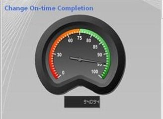
KPIs allow businesses to gauge the health of their enterprise and their performance by measuring their progress towards predefined goals. KPIs are business metrics that can be defined to monitor progress towards certain objectives and goals. A KPI will usually have a target and actual value, which will represent a quantitative goal that is critical to the success of the organization. KPIs are usually displayed on a scorecard, which contains a group of KPIs, to show the overall health of the business in one quick snapshot.
An example of a KPI is to complete all change requests within 48 hours. A KPI can be used to measure what percentage of change requests are resolved within that timeframe. The SM Dashboards represents the KPI visually. In the figure below, the KPI target value for completion of all change requests within 48 hours is 75%.
Partitions
A partition is a data structure that holds some or all of the data in a measure group. Every measure group is divided into partitions, which defines a subset of the fact data that is loaded into the measure group. Analysis Services Standard Edition only allows one partition per measure group, while Enterprise Edition allows a measure group to contain multiple partitions. Partitions are a feature that are transparent to the end user but will have a major impact on both performance and scalability of cubes. All partitions for a measure group will always exist in the same physical DB.
Partitions allow an administrator to better manage a cube and improve a cube’s performance. For example, you may remove or reprocess the data in one partition of a measure group without affecting the rest of the measure group. When loading new data into a fact table, only the partitions that should contain the new data are affected.
Partitioning also improves processing and query performance for cubes. Analysis Services can process multiple partitions in parallel, leading to a much more efficient use of CPU and memory resources on the server. While running a query, Analysis Services will fetch, process, and aggregate data from multiple partitions as well. Only partitions that contain data relevant to a query will be scanned, reducing the overall amount of IO needed.
One example of a partitioning strategy is to place the fact data for each month into a monthly partition. At the end of each month, all the new data will go into a new partition which will lead to a natural distribution of data with non-overlapping values.
Aggregations
Aggregations in a cube are a pre-summarized data sets and are analogous to a SQL SELECT statement with a GROUP BY clause. Analysis Services can use these aggregations when answering queries to reduce the amount of necessary calculations, returning the answers quickly to the user. Built-in aggregations in the cube reduce the amount of aggregation Analysis Services has to perform at query time. Building the correct aggregations can drastically improve query performance, and is often an evolving process throughout the lifetime of the cube as its queries and usage will change.
A base set of aggregations is usually created that will be useful for most of the queries against the cube. Aggregations are built for each partition of a cube within a measure group. When an aggregation is built, certain attributes of dimensions are included in the pre-summarized data set. Users will then be able to quickly query the data based on these aggregations when browsing the cube. Aggregations must be carefully designed because the number of potential aggregations is so large that building all of them would take an unreasonable amount of time and storage space.
The two options that SCSM DW team will leverage when building and designing aggregations in a SCSM OLAP cube:
1) Setting the “Performance Gain Reaches” option
2) Usage-based optimization
Performance Gain Reaches Option
The Performance Gain Reaches option defines what percentage of aggregations will be built. For example, setting this option to the default and recommended value of 30% means that aggregations will be built to give the cube a 30% estimated performance gain. Note that this does not mean that 30% of the possible aggregations will be built.
Usage-Based Optimization
Usage-based optimization allows Analysis Services to log the requests for data so that when a query is run, the information is fed into the aggregation design process. Analysis Services will then review the data and recommend which aggregations should be built to give the best estimated performance gain.
Here is an index list of the entire series:
- Part 1: OLAP Cubes in the SCSM Data Warehouse: Introduction
- Part 2: OLAP Cubes in the SCSM Data Warehouse : Key Concepts
- Part 3: OLAP Cubes in the SCSM Data Warehouse : Modeling the OLAP Cube in Management Packs
- Part 4: OLAP Cubes in the SCSM Data Warehouse : OLAP Cube Partitioning
- Part 5: OLAP Cubes in the SCSM Data Warehouse: OLAP Cube Processing
- Part 6: OLAP Cubes in the SCSM Data Warehouse: OLAP Cube Deployment
- Part 7: OLAP Cubes in the SCSM Data Warehouse: Troubleshooting
- Part 8: OLAP Cubes in the SCSM Data Warehouse : Maintenance and Administration