Forum Discussion
sum by color when colors are set by conditional formatting
- Jan 19, 2017
Hi matt nipper,
since you mentioned that you "have done an exhaustive search online" i have come up with a solution for you, although it has two limitations A) it will only work, if your rules of conditional formatting is created using conditional formatting rules with formula aka (use a formula to determine which cells to format) and B) the UDF will only work if sum range is more than one cell another word, it will not sum a single cell, as well as the conditional formatted range is more than one cell.
the example file, you can download it from here. I could not upload it here, as it is a Excel Macro-enabled Workbook that contains the UDF
Function SumConditionColorCells(CellsRange As Range, ColorRng As Range)
Dim Bambo As Boolean
Dim dbw As String
Dim CFCELL As Range
Dim CF1 As Single
Dim CF2 As Double
Dim CF3 As Long
Bambo = False
For CF1 = 1 To CellsRange.FormatConditions.Count
If CellsRange.FormatConditions(CF1).Interior.ColorIndex = ColorRng.Interior.ColorIndex Then
Bambo = True
Exit For
End If
Next CF1
CF2 = 0
CF3 = 0
If Bambo = True Then
For Each CFCELL In CellsRange
dbw = CFCELL.FormatConditions(CF1).Formula1
dbw = Application.ConvertFormula(dbw, xlA1, xlR1C1)
dbw = Application.ConvertFormula(dbw, xlR1C1, xlA1, , ActiveCell.Resize(CellsRange.Rows.Count, CellsRange.Columns.Count).Cells(CF3 + 1))
If Evaluate(dbw) = True Then CF2 = CF2 + CFCELL.Value
CF3 = CF3 + 1
Next CFCELL
Else
SumConditionColorCells = "NO-COLOR"
Exit Function
End If
SumConditionColorCells = CF2
End Function
in the attached example file you can see that from A3:G16 cells are formatted using Conditional Formatting.
User Defined Function (UDF) is placed in cells J2 & J3 and cells I2 and I3 are the criteria color used as reference inside the UDF in J2 and J3.
I hope this helps you.
Edit: uploaded file and updated the code to the correct one.
Hello!
Do you have a sample excel file where you use the count by conditional format?
I am having problems using it.
Thanks!
Hello Bethany,
Yes, I have attached it here.
- JamilFeb 13, 2019Bronze ContributorHi Julius835,
As you can see in my earlier post. The range inside UDF and the range of CF both must be the same, otherwise the UDF does not count. Perhaps It would be easier if you use SUMPRODUCT function to count conditionally based on multiple criteria.
Put a helper column next to column E. you can hide that if you want. put real dates in them and then use something like =SUMPRODUCT(--(MONTH(F:F)=MONTH(TODAY())),--(YEAR(F:F)=YEAR(TODAY())))  Julius835Jan 16, 2019Copper Contributor
Jamil,
Thank you for your response. I have made the necessary changes and now my issue is if I try to count the cells only in certain rows I get an incorrect number.
- JamilJan 16, 2019Bronze Contributor
Hi Julius835,
There are several issues with your workbook that is why UDF result in error.
I thought, I could explain it better by recording a video. Please see attached workbook and the video.
- Julius835Jan 16, 2019Copper Contributor
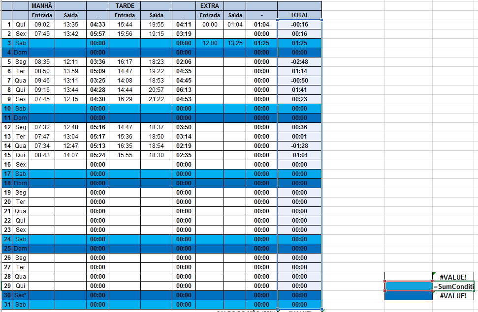
Hi Jamil, I believe I've done everything properly yet it still displays "#VALUE!" please help me.
- JamilDec 07, 2018Bronze ContributorHi
If you read my earlier posts. you will see that I mentioned that for the UDF to work. CF needs to be creating using formula. I checked your CFs are not creating using Formula and that is why it does not work. If you change your CFs to be based on formula then it will work.  electricrickDec 07, 2018Copper Contributor
Hi Jamil,
I have tried everything and even inserted my sheet into your uploaded file but the count colours function only returns 0
Please help
- JamilNov 20, 2018Bronze ContributorZ Z
Glad to hear that it works. Have a wonderful day too. thx for the feedback.  Z ZNov 20, 2018Copper Contributor
Jamil,
Thank you!!!!! It works as I needed it.
Have a wonderful day.
- JamilNov 19, 2018Bronze Contributor
Hi Z Z,
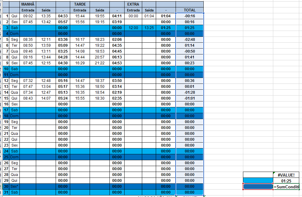
Your conditional formatted area was not exactly as per your range used in the UDF.
If you want to count per row, then your CF should be per row. I have modified the CF and now it works.
plz see attached.
- Z ZNov 18, 2018Copper Contributor
Hello Jamil, Can you please help? I need to count all cells in a range (row or column, but in this case is a row) that have been conditionally colored. I tried following your instructions but I get "0". I have 6 (six) clusters of data (ranges) which I have assigned a range name. The conditional formatting formula finds all cells which value repeats in all clusters (if the number does not repeat in ALL clusters then the cell does not get highlighted). I need to COUNT per row how many cells are highlighted, and I have to be able to do the same with all rows individually. Please see attached file. Can you do it in my file and explain what is wrong? Thank you Jamil.
- JamilJul 28, 2018Bronze ContributorYes. please see my example here
https://techcommunity.microsoft.com/t5/Excel/sum-by-color-when-colors-are-set-by-conditional-formatting/m-p/174923/highlight/true#M8275  amin ahmadiJul 11, 2018Copper Contributor
hi, tnx for your file. is it possible to count color of conditional formatting cells in excel with vba only for those cells which are only numberic?
- JamilMar 27, 2018Bronze ContributorHi Cara,
I looked the file you attached. there were many issues that probably caused that error.
A) The workbook had No UDF in it. hence NAME? Error
B) this UDF has two limitations 1- it will only work, if your rules of conditional formatting is created using conditional formatting rules with formula aka (use a formula to determine which cells to format) and I could see in the workbook you shared that there were two rules which was not determined by formula 2- Second the UDF will only work if sum range is more than one cell in another word, it will not sum a single cell or if Conditional formatting rule is applied in range that is a single cell. In your workbook there were multiple rules that applied in single cells.
As I suggested in my earlier posts, If the UDF works, then fine, if does not work then it is not the only and optimal solution. So, rather than Counting based on the outcome of the conditional formatting, you can use the same criteria as exists in the conditional formatting to Count the cells using COUNTIFS or SUMPRODUCT
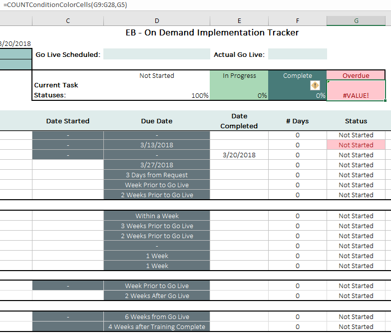
I didn't examine in in depth your workbook as the data validation were linked to another workbook and for me it was showing a broken link. You could use the conditional formula to return values in column G and based on the values you could simply count the overdues with simply formula like this =COUNTIF(G9:G28,G5) - Cara PfaffMar 26, 2018Copper Contributor
Still getting the same error, thank you for taking a look, it's attached.
- JamilMar 22, 2018Bronze Contributor
Sometimes this happens, if you have an external Add-in or there are some codes in the PERSONAL.XLSB workbook.
click on the cell that has #Value error and then press F2 to go to Edit mode and then enter again. if you see the VALUE error disappear that means that the error is caused by some external add-in or your personal.xlsb workbook that is in the start up folder.If you can share a dummy example file, I can take a look at it.
- Cara PfaffMar 21, 2018Copper Contributor
Hi! I've also been getting the #Value error. I copied and pasted the Count version of the VBA. Screen shot attached let me know if you need more. I entered the RGB color codes so they are exact.
- JamilMar 19, 2018Bronze ContributorCan you post a screenshot of dummy data or a dummy excel file?
- Joshua StoneMar 19, 2018Copper Contributor
When I use the code, it shows #VALUE!. This is happening once the condition changes.
I am using Excel 2016 with Windows 10 Pro.
- JamilMar 19, 2018Bronze Contributor"does this work for the color WHITE as well? "
There are two things not to mixup the WHITE background color with No-Background Color.
If your cells have conditional formatting and the color is selected is plaint white then yes it works. but if the cells have No color meaning it the background color is None then it does not work.
RE: on your second question:
you need to check the colors of your conditionally formatted cells and the color of criteria. they must match 100%. sometimes, the colors look similar while they are different, best way to guarantee you are using the exact same color is to find that specific color's color code and that you can do by using VBA to find the color code of your cells.
If you do not want to go in that direction then i suggest you rebuild your conditional formatting cells by selecting a simple color and then also use the same color in the criteria cell.
in case if you wanted to find out the color code with VBA then here is a link https://www.thespreadsheetguru.com/the-code-vault/2014/11/5/retrieve-excel-cells-font-fill-rgb-color-code that explains how. - Hewdy LopesMar 15, 2018Copper Contributor
On your worksheet all the colors work just fine. But on mines, for some reason only 1 out of 3 colors i'm using works, the light blue. Those columns that are highlighted are conditionally formatted using a formula.
I've made 3 sample formula for each of the colors.
- Hewdy LopesMar 15, 2018Copper ContributorJamil, does this work for the color WHITE as well? i seem to get the error "#VALUE!" when using the SumConditionColorCells formula. Other colors seems to work.