XLOOKUP partial match text

[Kristin2185]

Hi, 

I'm having an issue with partial matching text in the lookup cell of my X lookup function.

Formula:

=XLOOKUP("*"&A2&"*";$I$6:$I$13;$J$6:$J$13;"not found";2) 

A2 = app:android:sv:code=0

Lookup array has "app" as value (I13) (though written without "", ie app) and return array value is also app (J13). 

I only get "not found" as output when executing this formula. I want the output to be "app" for A2 in the output cell. 

I'm on a Mac, Swedish computer with English language Excel. 

What can I do??

[#2]

Hi @Kristin2185,

You can do that with the FILTER function.

I combined it with the TAKE function here in case there are more than one partial match, then it will only return the first match.

=TAKE(FILTER($J$6:$J$13,IFERROR(FIND($I$6:$I$13,A2),0)=1,"not found"),1)

Regards,

Zach

[#3]

Hi @Zach Prins 

Thanks for your reply! 

I tried your formula without much success, unfortunately. 

See attached my spreadsheet (my wanted outcome is exemplified in column D (I want all cells to populate with the text in J6:J13 when they match the list in I6:I13))

Should the formula you suggested still work or will I need to do something differently? 

Best, 

Kristin

[#4]

Aha, I should've started off asking whether the dynamic array formulas are available in your version of Office. Are you using Office365? If so the formula should work as is if copied into cell C2

[#5]

@Zach Prins 

I use Office365, on a MacBook.
Got the wanted results now, thank you so much!!

I think the issue was that this formula populates two columns with data and so I got a #spill error that I didn't understand. Worked perfectly when I made sure there were two empty columns available.  

[#6]

Although... In row 18, the formula doesn't catch the "fb-rem" in the middle of the string. Any ideas on how to address that?

[#7 · Accepted solution]

Hi @Kristin2185 

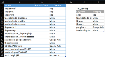
Slightly different approach that should work if your Source strings are as consistant as those you shared where there's a semi-column following the keywords you want to match

in C2:

=FILTER(TBL_Lookup[Mapping], ISNUMBER(SEARCH(TBL_Lookup[Keyword],A2)), "No match")

[#8]

@Kristin2185, in that first reference of your formula you're referencing columns I and J, it should be only column J.

=TAKE(FILTER($J$6:$J$13... 

[#9]

Thanks, this works perfectly!

[#10]

@Kristin2185 

Glad @Zach Prins & I could help & Thanks for providing feedback

Nice week-end...