XLOOKUP on several rows and columns

[Martin_Gemen]

Hi All,
I want to use XLOOKUP on several rows and columns, but that does not seem to work.

=XLOOKUP(F10:F357,Q10:T96,Q9:T9)

Range F10:F357 contains numbers that can be found in Q10:T96 as well.

Depending on the position of lookup value it should return the respective header which is contained in range Q9:T9.

Unfortunately this does not work as XLOOKUP cannot work on arrays (rows >1, columns >1).

Does anybody have a solution for this?
Thanks in advance.

Best regards,

Martin

[#2 · Accepted solution]

@Martin_Gemen 

In G10:

=INDEX($Q$9:$T$9,SUMPRODUCT(($Q$10:$T$96=F10)*COLUMN($Q$10:$T$10))-COLUMN($Q$10)+1)

Fill down to G357.

[#3]

@Martin_Gemen 

The same result is returned with this formula:

=IFERROR(INDEX({"A"."B"."C"."D"},SUMPRODUCT(MMULT(N($Q$10:$T$96=F10),TRANSPOSE(COLUMN(Q:T))))-16),"")

or

=IFERROR(INDEX($Q$9:$T$9,SUMPRODUCT(MMULT(N($Q$10:$T$96=F10),TRANSPOSE(COLUMN(Q:T))))-16),"")

[#4]

@Hans Vogelaar
Thanks a lot for your provided solution.
To have only one formula for the range F10:F357, I changed it to
=BYROW(F10:F357,LAMBDA(array,INDEX($Q$9:$T$9,SUMPRODUCT(($Q$10:$T$96=array)*COLUMN($Q$10:$T$10))-COLUMN($Q$10)+1)))

[#5]

@Quadruple_Pawn
Thanks a lot for your provided solution.
The first one did not work in my case. The part ... {"A"."B"."C"."D"} is not recognized.
The second one did work.
For now I go for the other posted solution.

[#6]

@Martin_Gemen 

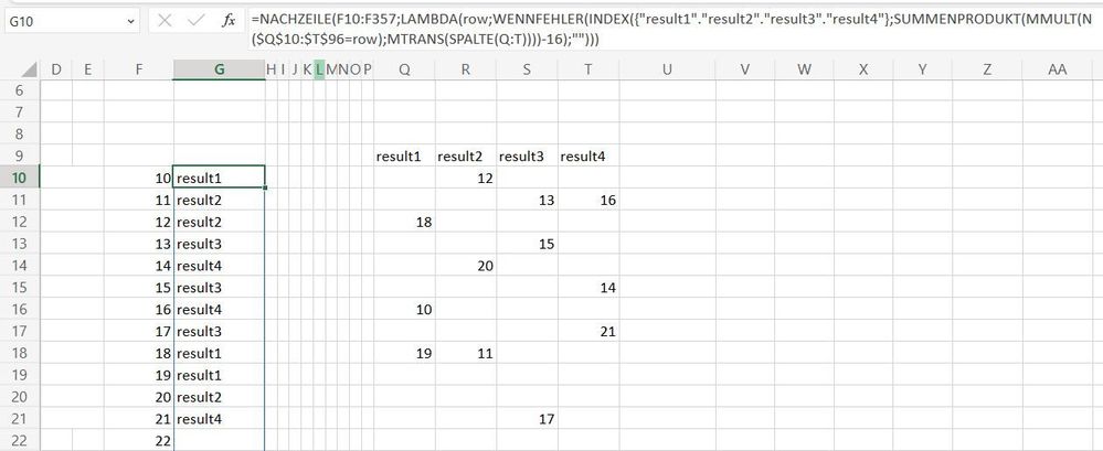
You are welcome. I should have mentioned that {"A"."B"."C"."D"} has to be replaced with the values from range $Q$9:$T$9 as shown in the example in the screenshot e.g. {"result1"."result2"."result3"."result4"}.

=BYROW(F10:F357,LAMBDA(row,IFERROR(INDEX({"result1"."result2"."result3"."result4"},SUMPRODUCT(MMULT(N($Q$10:$T$96=row),TRANSPOSE(COLUMN(Q:T))))-16),"")))

[#7]

@Quadruple_Pawn
Ah, Ok. Thanks for your update.
Best regards,
Martin