What formula to use for multiplying countifs result?

[little2fern]

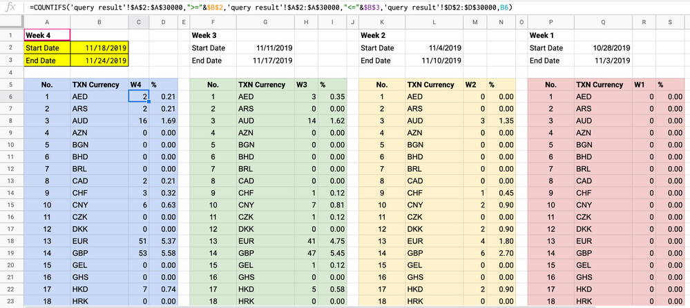
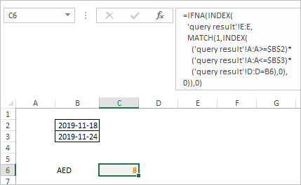
Here is my current formula of C6. I need a new formula for C6 and my goal here is to

- find out how many time 'AED' in cell B6 appears (in spreadsheet 'query result') within the selected dates of cell B2 and B3

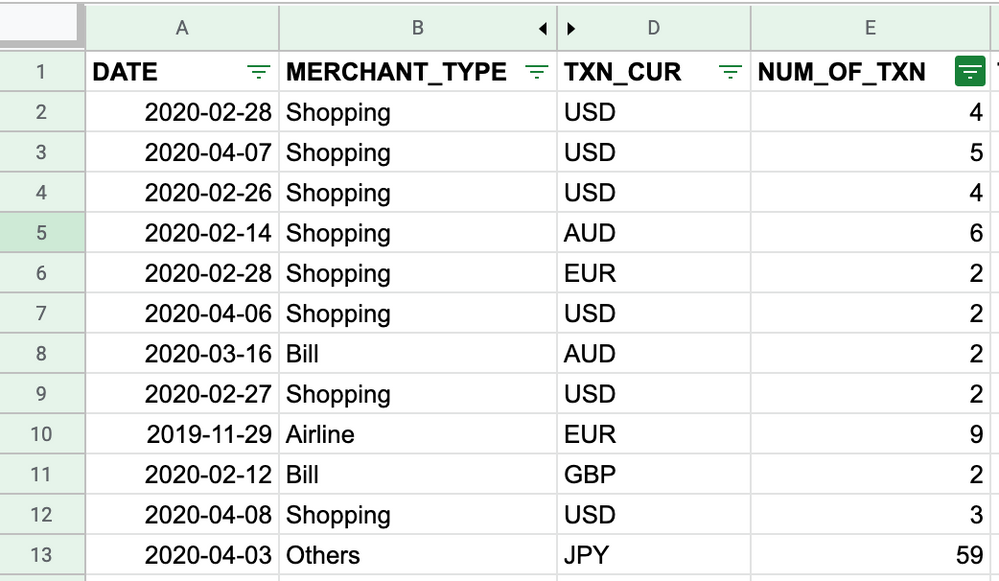
- also after finding out how many times AED appears, I need to multiply the count by the number appear in E column called NUM_OF_TXN (in spreadsheet 'query result').

Attachment 1: where new formula in C6 needs to be

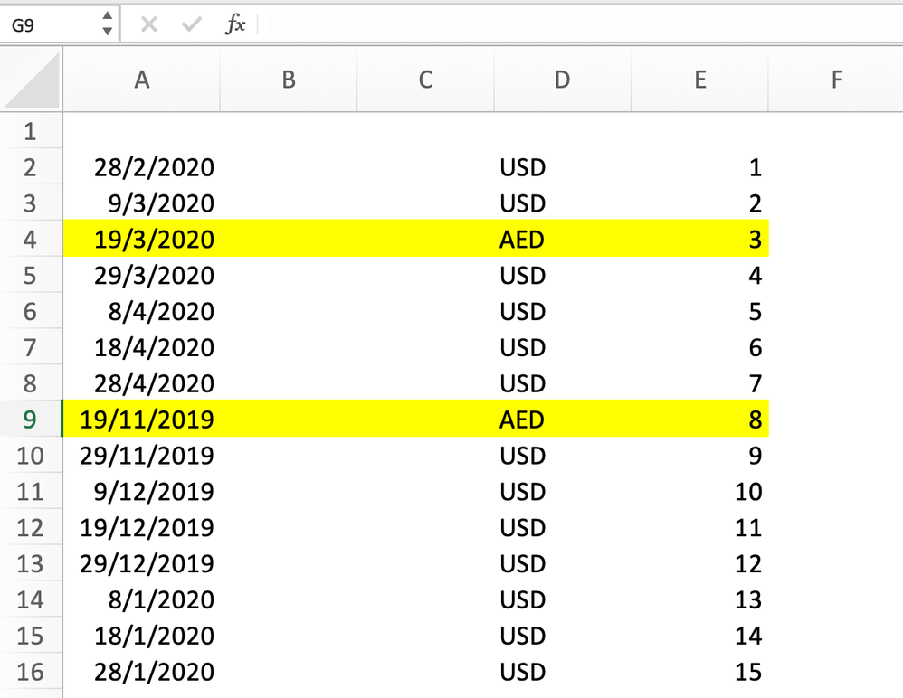
Attachment 2: source the formula refers to spreadsheet called, 'query result'.

[#2]

@little2fern 

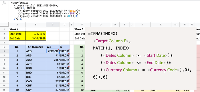
I guess the first part with COUNTIFS works. To find the number form column E you may use INDEX/MATCH assuming first found number for given date range will be taken (if it could be few of them). Formula could be like

=IFNA(INDEX(
  <Target Column E>, 
  MATCH(1, INDEX(
     (<Dates Column> >= <Start Date>)*
     (<Dates Column> <= <End Date>)*
     (<Currency Column> = <Currency Code>),0),
  0)),0)

We return zero if nothing was found.

[#3]

@Sergei Baklan 

<Target Column E> means NUM_OF_TXN in column E of spreadsheet query result

<Currency Column> means TXN Currency in column B

<Currency Code> means TXN_CUR in column D of spreadsheet query result

Correct?

[#4]

@little2fern 

Not exactly. Currency column is

and Currency Code is "AED" or like.

[#5]

@Sergei Baklan 

Thanks.

I tried the formula below both in excel and google sheets, but it still doesn't work.

The error says, 'Formula parse error'.

=IFNA(INDEX(
  <'query result'!$E$2:$E$30000>, 
  MATCH(1, INDEX(
     (<'query result'!$A$2:$A$30000> >= <$B$2>)*
     (<'query result'!$A$2:$A$30000> <= <$B$3>)*
     (<'query result'!$D$2:$D$30000> = <B6>),0),
  0)),0)

I think it would be easier if I share the file with you.

Can I have your gmail address please? The file is in Google Sheets.

[#6]

@little2fern 

I emulated that in the attached file

In your formulas just remove placeholders signs < >.

[#7]

@Sergei Baklan 

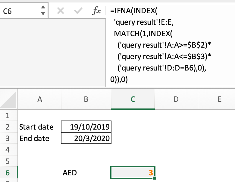
I tried removing the <> and it works, however the result isn't what I expect to see.

In your query result spreadsheet, there're two AED results shown in D4 and D9. This means that the sum of AED appearing in between start date 19/10/2019 and end date 20/03/2020 should be (8+3) = 11. 

However this formula shows the result as 3 instead of 11.

What formula should I use in this case?

Thank you,

Fern

[#8 · Accepted solution]

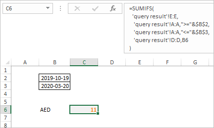
@little2fern 

If to sum that will be another task, formula for it is

=SUMIFS(
  'query result'!E:E,
   'query result'!A:A,">="&$B$2,
   'query result'!A:A,"<="&$B$3,
   'query result'!D:D,B6
)

as here

[#9]

@Sergei Baklan 

Yes! The results are displaying the correct data.

Thank you so much, Sergei.

[#10]

@little2fern , you are welcome, glad to help