Weighted Average with multiple criteria and looking for specific name

[Deleted]

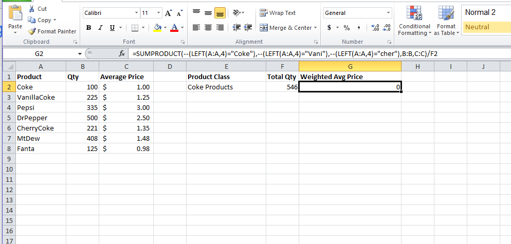
Hi, I'm trying to figure out how to get the weighted average price of multiple products within the same class.  For example see the sheet below.  I want to find the weighted average price of all coke products, ie Coke/VanillaCoke/CherryCoke. 

The formula I have tried is:

=SUMPRODUCT(--(LEFT(A:A,4)="Coke"),--(LEFT(A:A,4)="Vani"),--(LEFT(A:A,4)="cher"),B:B,C:C)/F2

This doesn't work.  Please help!!

[#2 · Accepted solution]

Hi Blake,

Please try this formula:

=AVERAGE(AVERAGEIFS(D2:D8, A2:A8,{"Coke","VanillaCoke","CherryCoke"}))

With this formula, you don't have to manually calculate the Qty.

But the best way is to create another column in the table to hold the class for each product.

This will make the calculation easier so that you don't have to hard-code each product in the formula.

This can be done as follows:

Please find the attached workbook

Hope that helps

[#3]

@Haytham Amairah 

This example/solution is just the simple average and not the weighted average.  The calc for weighted average is as attached and would need a column with total cost per item calculated (cost per unit X units).  This column can then be hidden for presentation purposes if desired.

[#4]

With regards to your original formula, why not add a column to your table for product class (I think someone else may have suggested this already)? I would use a data validation drop down to make it easier and to avoid spelling errors. But, if you had product class in column A (I would not use the entire column as you'll likely get an error trying when sumproduct tries to multiply text - perhaps consider using a structured table):

=SUMPRODUCT(--(A2:A100=E2),B2:B100,C2:C100)/F2

And F2 is

=SUMPRODUCT(--(A2:A100=E2),B2:B100)

Also, you would add items that are OR conditions instead of multiplying (which is AND), but this is just for your information - I would suggest adding the product categories column.

=SUMPRODUCT((LEFT(A2:A100,4)="Coke")+(LEFT(A2:A100,4)="Vani")+(LEFT(A2:A100,4)="cher"),B2:B100,C2:C100)