- Home
- Microsoft 365
- Excel
- Re: Want to make 1 autoupdate worksheet from downloaded daily transaction reports in CSV files
Want to make 1 autoupdate worksheet from downloaded daily transaction reports in CSV files
- Subscribe to RSS Feed
- Mark Discussion as New
- Mark Discussion as Read
- Pin this Discussion for Current User
- Bookmark
- Subscribe
- Printer Friendly Page
- Mark as New
- Bookmark
- Subscribe
- Mute
- Subscribe to RSS Feed
- Permalink
- Report Inappropriate Content
Sep 20 2022 10:35 AM
Hi All,
iam using MS Office 2019, I download daily transaction reports in CSV format in a single folder with name as current date like (26122022.csv), there is so many type of transactions like Money Transfer, Recharge, Bill..etc, and these transaction are with Fail, Refund, Success Status, I want to make a Master Worksheet which show Sum of each type of transaction Amount with success status and when I apply same formula on next cell source file name automatically change according to date show in first column in master sheet, kindly suggest what can i do to create sheet.
Regards
SK Grewal
- Mark as New
- Bookmark
- Subscribe
- Mute
- Subscribe to RSS Feed
- Permalink
- Report Inappropriate Content
Sep 21 2022 12:14 AM
for obvious reasons, I cannot provide a fully detailed explanation on how to achieve your needs. But I hope the following steps will point you into the right direction:
To import your CSV files into your workbook, use Power Query (menu "Data | From Text/CSV"). Select the file and check the structure of it in the preview window. If the file has already the correct structure and you really need all columns, you can load it directly into an Excel worksheet. Otherwise, chose "Transform Data". This will open the Power Query Editor, where you can do all types of data cleansing and transformation. Once you are finished there, close & load the query into a worksheet.
Next, choose an empty cell somewhere in your workbook, preferable put it above your loaded data table. In this cell, enter the complete path and file name of the CSV file that you import. Then give this cell a name (menu "Formulas | Define Name"), e.g. "Sourcefile"
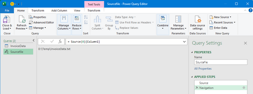
Select this named cell and load it into Power Query (menu "Data | From Table/Range"). In the Power Query editor, this query will most likely have three applied steps: Source, Promoted Headers and Changed Type. Delete all steps apart from the first one ("Source"). Now you should see the path and filename that you have entered in your named cell, and also a header "Column1". Now do a right click directly on the path/file name and choose "Drilldown". As a result, you should see only a text string with the path and file name:
Next, select the query with your imported CSV file (in my example "InvoiceData"). In the list of applied steps, highlight the first one "Source". In the formula bar above the table, you should see a formula that contains hardcoded the path and file name to your source file:
Replace that hardcoded string with the name ouf your second query (in my example "SourceFile"), but do not mess around with the rest of the formula:
In the preview table, nothing should have changed. The only difference is, that the source file can now change dynamically, based on what you enter in the named cell in your worksheet.
Now close the Power Query editor. In Excel, you can now change the path and name of the source file to the new location/name, then do a right-click in the currently loaded data table and choose "Refresh":
If everything works fine, you should now get the new data loaded after a few seconds.
Now you can build Pivot tables on your loaded table for any sort of analysis.
There are ways to use a date field as a parameter for the import, but this requires more sophisticated transformations in Power Query.


