- Subscribe to RSS Feed
- Mark Discussion as New
- Mark Discussion as Read
- Pin this Discussion for Current User
- Bookmark
- Subscribe
- Printer Friendly Page
- Mark as New
- Bookmark
- Subscribe
- Mute
- Subscribe to RSS Feed
- Permalink
- Report Inappropriate Content
Jan 26 2022 09:11 AM - edited Jan 26 2022 09:14 AM
I use Excel version 2112. I have a list of College names that I search for to return a value that 
I use =VLOOKUP(B7,DEVIATION!A:D,3,FALSE) and as stated it pulls all correct data but only those with a singular name. I am almost 80 and have no experience with excel., but attempting to learn. Thanks for your help. Email address removed
- Labels:
-
Excel
-
Office 365
- Mark as New
- Bookmark
- Subscribe
- Mute
- Subscribe to RSS Feed
- Permalink
- Report Inappropriate Content
Jan 26 2022 11:27 PM
Can only commend you that you want to learn new things! Since you mention to be using Office365, your Excel version should support the new dynamic array functions. On of these is FILTER. Combined with ISNUMBER and SEARC, you can extract all information from a structured table, based on a partial search phrase. Attached a file demonstrating it. See if you can get started with this on your own. If not, come back here.
- Mark as New
- Bookmark
- Subscribe
- Mute
- Subscribe to RSS Feed
- Permalink
- Report Inappropriate Content
Jan 27 2022 03:32 PM
Riny,
I don't have words to express my Thanks to you for your time and assistance. Many people these days don't help. I am very proud to make your acquaintance. However, I will waste no more of your time with this. My filter icon does not offer the same choices as yours. Even though I highlighted many areas for filtering I got the same -no results-no choices. I then attempted to input your formula changing to my cells, but again I failed to achieve results. To complicate matters I have two columns of data to extract when the college is chosen thus creating a false in the formula depending on which column I am asking for. To understand I seek standard deviation that I have already computed depending on whether the team is home or away when playing basketball. I am stumped, but will live with it for now. Keep helping others, it comes back with large rewards! Steve
- Mark as New
- Bookmark
- Subscribe
- Mute
- Subscribe to RSS Feed
- Permalink
- Report Inappropriate Content
Jan 27 2022 10:19 PM
@steve560 Always glad to help, and I will not give up yet.
You wrote "My filter icon does not offer the same choices as yours." Well, that's because the FILTER I'm talking about is a function, i.e. not related to a button or an icon.
When you look in cell G5, you'll see it contains this formula:
=FILTER(Table1,ISNUMBER(SEARCH(F5,Table1[College])))It filters out all rows from the table (Table1) where a search for the keyword (in F5) in the College column of Table1 results in a number. Looking into each of the functions used (the ones in blue above) separately you'll get this:
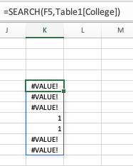
The SEARCH function returns an array with value errors (keyword not found) and numbers (keyword found).
ISNUMBER returns an array of Trues and False, depending on what's in the outcome of SEARCH (in this example referred to as K5# because that where the SEARCH array is located and the # means it picks up the entire array).
Now, the FILTER function picks-up all the rows in Table1, where it finds TRUE in the ISNUMBER step (i.e. the 4th and the 5th row.
When you study the FILTER function further you will note that you can use more than one filter criteria.
For instance, you could use:
=FILTER(Table1,(ISNUMBER(SEARCH(F5,Table1[College])))*(Table1[Value]>4))Put each criteria in it's own set of brackets and use * to apply a logical AND or + to apply a logical OR. This example will only return the 5th row as it is the only one with "colo" in the College column AND a value greater than 4 in the Value column.
- Mark as New
- Bookmark
- Subscribe
- Mute
- Subscribe to RSS Feed
- Permalink
- Report Inappropriate Content
Jan 31 2022 05:54 AM
- Mark as New
- Bookmark
- Subscribe
- Mute
- Subscribe to RSS Feed
- Permalink
- Report Inappropriate Content


