VLOOKUP show wrong values

[Radoslavov91]

Hi all, i have the following problem with an excel function.

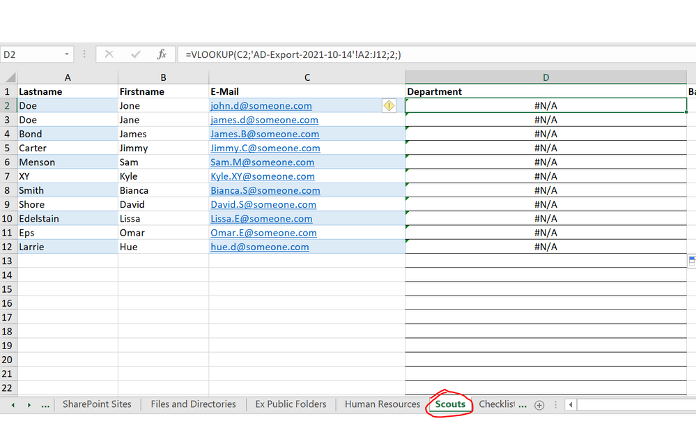
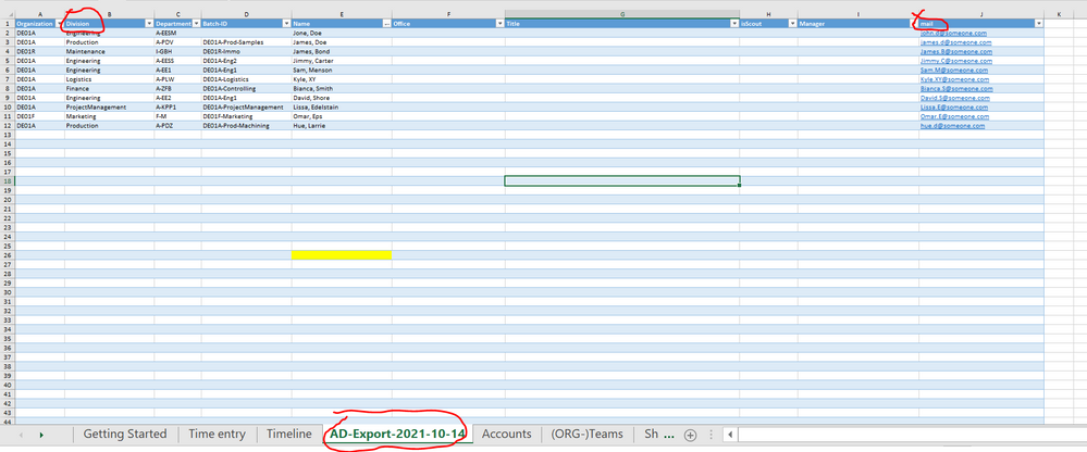
I have a file with two sheets, sheet one (AD-Export) contains data for the employees (such as first name, email, department) and the second sheet (Members) contains a list of members (First name, email, department). I'm using the VLOOKUP formula every time when a new user is added in the Members sheet, to search by its email in the AD-Export one and fills out automatically the department.

The formula is like this: =VLOOKUP(C3;Table1;2;FALSE)

The problem is that the information in the table_array is correct, but the formula returns #N/A -

Value Not Available Error

A value is not available to the formula or function.

I don't know what I'm doing wrong, as it should be fairly simple formula.

thanks in advanced

Kiril

[#2]

@Radoslavov91 

It's difficult to read the details in your attached files but i guess the formula should be like:

=VLOOKUP(C3;Table1!B2:C10;2;FALSE)

if the name of the table is Table1. If it's AD-Export then try

=VLOOKUP(C3;'AD-Export'!B2:C10;2;FALSE)

[#3]

@Radoslavov91 

Your VLOOKUP formula looks up C3, i.e. the email address, in the first column of Table1.

But the first column of Table1 that is visible in your screenshot is Division. Does Table1 begin in column A? If so, you should have included it in the screenshot.

Better attach a stripped-down copy of the workbook with some dummy data.

[#4]

@Hans Vogelaar here is a new screenshot with sample data, and again is not working :(

Regards

[#5]

I've missed to add the formula as well: =VLOOKUP(C2;'AD-Export-2021-10-14'!A2:J12;2;FALSE)

[#6]

@Radoslavov91 

VLOOKUP doesn't work to the left

[#7]

@Radoslavov91 

=VLOOKUP(C2,CHOOSE({1,2},'AD-Export-2021-10-14'!$J$2:$J$14,'AD-Export-2021-10-14'!$B$2:$B$14),2,FALSE)

You want vlookup to the left. Please enter this formula as arrayformula with ctrl+shift+enter.

[#8]

@Radoslavov91 

VLOOKUP always searches for the lookup value in the first column of the range.

Use

=IFERROR(INDEX('AD-Export-2021-10-14'!$B$2:$B$12, MATCH(C2, 'AD-Export-2021-10-14'!$J$2:$J$12, 0)), "")

[#9]

@Hans Vogelaar I'm uploading a copy of the file with some sample data

Neither of the proposed formulas worked, unfortunately i don't want to rearrange the columns in AD Export sheet as there are other sheets from the file that are referring to this sheet and they have formulas that might break.

regards

[#10 · Accepted solution]

@Radoslavov91 

As @Hans Vogelaar suggested

=IFNA( INDEX(Table1[Batch-ID], MATCH(Scouts!C2, Table1[mail], 0) ), "no such")

[#11]

@Radoslavov91 

The suggested formula work fine. Please see attached file.

[#12]

Thank you Sergei, and the rest of the people spare time to help me.

It worked, i was just wondering what it was so complex the whole formula, I've watched so many tutorials on using VLOOKUP and they were fairly simple, but in my case that wasn't the situation i guess .

Thank you all again, stay safe!

Regards
Kiril

[#13]

@Radoslavov91 

That was one of few reasons why XLOOKUP() was introduced - VLOOKUP() works only to the right and use fixed returned column number; INDEX/MATCH looks bit complex for many users. 

[#14]

I am having a similar issue. I am can't seem to post photos but I would if it was possible. I am trying to use the Vlookup for dates but when i do this I get a #Value error.

[#15]

@JoshGold 

That's better to discuss with sample file. Perhaps you have texts which looks like dates, not actual dates which in Excel are numbers in behind.