VLOOKUP Return Multiple Results

[jharrisgray]

Hello All,

I wanted to see if someone could assist me with a sheet I'm currently working on.  Basically I have a excel sheet with multiple sheets.  I have a sheet named "Master" then 3 other sheets.  On the master sheet what I'm trying to accomplish is a vlookup to look for a value on the master sheet on all 3 of the other sheets and return the sheet name as the value.  I can get this to work fine if just using a VLOOKUP for 1 sheet at a time, but what I'm looking for is to return the sheet name of all sheets that the value is present in on the master sheet.  I've attached the sheet for reference and in short what I want the lookup to do is:

* Result should be listed on Master sheet, field G4

* Formula entered on this field will look on all other sheets for the value in Master C4 (AA:AA:AA:AA:AA:AA)

* On this example, you can go to all sheets and see that I've listed this value on all 3 sheets

* The result from the formula should list the B column values from all other sheets, in this case since the C4 value is on all 3 worksheets there should be 3 different results listed. So the formula should list the results as "10.2.2.1 - 10.2.2.2 - 10.2.2.3"

Any help would be greatly appreciative! 

[#2 · Accepted solution]

@jharrisgray 

Unless I'm mistaken, to get exactly what you're asking for, you're going to need Power Query or a tool like that; sadly, I'm not experienced with that.

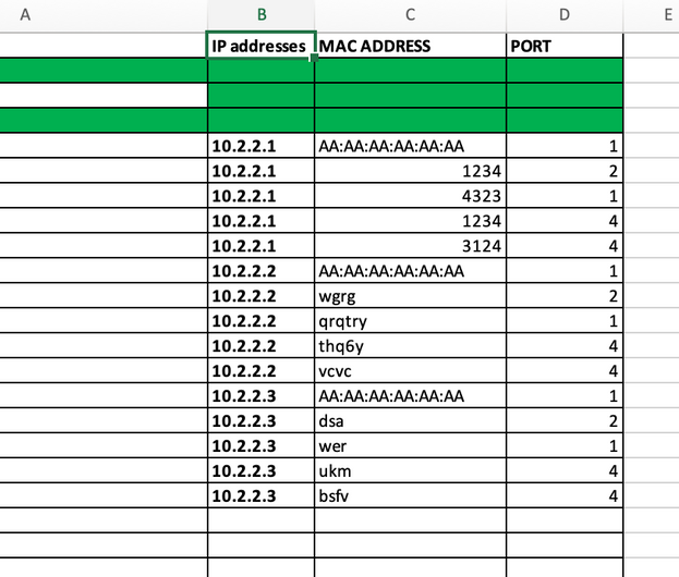
However, I am experienced with databases and database design, and I'm questioning why you have three separate sheets for the subordinate data here. One could suffice, I believe, recognizing that column B in those sheets is redundant with the name affixed to the tab. Just let that column do the differentiating that the tab is doing.

(An aside: we often create separate pages because that's how we'd do it on paper, but the reality is that such a layout actually (often) interferes with Excel's marvelous abilities to parse such distinct entities in a single database or table, just using a column to differentiate what was originally presented as separate tabs.)

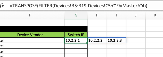
When you do that--as I've done in the demo attached--then a simple FILTER function, nested in TRANSPOSE, gives you the desired result, albeit in three separate columns, G, H and I.

[#3]

Thanks for the response Mathetes. Yeah I see what you're saying. The actual document I'm working on has 15 tabs with thousands of lines of information, I just made this little sheet as a example template. But I didn't think about transpose with a filter, was just planning on vlookup, but this works as well. With that solution is there a way to make all results list in only the field the formulas entered instead of going out into the next fields (Like a word wrap)?

[#4]

Disregard Mathetes, I found a way to do it with a additional TEXTJOIN formula. Appreciate all the help!

[#5]

@jharrisgray 

Something like this?

=TEXTJOIN(" -- ",1,FILTER(Devices!B5:B19,Devices!C5:C19=Master!C4))

That's so neat. Thank you for pointing me to that refinement. I've not used TEXTJOIN before; it's a great enhancement to some applications of the FILTER function, since that function produces an array. For a limited array, this would at times be very useful indeed.