- Home
- Microsoft 365
- Excel
- Re: VLOOKUP PULLING TOTAL SUM FROM A MULTIPLE RAWS
VLOOKUP PULLING TOTAL SUM FROM A MULTIPLE RAWS
- Subscribe to RSS Feed
- Mark Discussion as New
- Mark Discussion as Read
- Pin this Discussion for Current User
- Bookmark
- Subscribe
- Printer Friendly Page
- Mark as New
- Bookmark
- Subscribe
- Mute
- Subscribe to RSS Feed
- Permalink
- Report Inappropriate Content
Sep 15 2022 07:16 PM
Hello there. Need help pls.
I want to know, how I can pull out the total SUM of multiple rows by VLOOKUP. With VLOOKUP, I look up for the value (Example Invoice number ADL01) in sheet 1 and pull the Line value from sheet 2 belongs to ADL01 invoice number. But what if, sheet 2, has multiple rows with same Invoice number ADL01 and I want to pull the TOTAL SUM of those multiple rows in sheet 2 to sheet 1 with VLOOKUP? Any help pls. Thanks.
- Labels:
-
Excel
- Mark as New
- Bookmark
- Subscribe
- Mute
- Subscribe to RSS Feed
- Permalink
- Report Inappropriate Content
Sep 15 2022 07:50 PM
@RohanAbaHK Then you can use SUMIF.
- Mark as New
- Bookmark
- Subscribe
- Mute
- Subscribe to RSS Feed
- Permalink
- Report Inappropriate Content
Sep 15 2022 08:01 PM
@RohanAbaHK Not completely sure what you are aiming to do, but from my understanding look at the example below for a recruitment service.
| candidate_name | application_id | assigned_value |
| John | A1 | 1 |
| Cam | A6 | 1 |
| Simon | A1 | 1 |
| Jenny | A3 | 1 |
The above table has distinct candidate_name in the 1st column, although there are multiple application_id. To get a total count of applications for each candidate, assign '1' as a value to each row on a new column (In this example the new column is assigned_value).
Use vlookup to and select the whole table in this case. It'll assign the correct application_id next to the candidate_name based on sheet1.
After that step, click on an empty cell anywhere and navigate to the 'data' tab. Then click on 'Consolidate' and select the entire table as in the above case we need to look up total applications for distinct candidates. Once you have selected the range, then click on 'add' within the 'consolidate' dialog box and then tick the 2 boxes, 'top row' and 'left column' and finally click on consolidate. Ensure to select 'sum' in the dialog box.
What this does is calculates the total applications for each distinct candidate. The top row contains the headers of the table and the left column is used to look up the total for each distinct customer.
It'll be more helpful if you could include an example of what it is you're trying to achieve with vlookup and provide an example as well. Hope this helps!
- Mark as New
- Bookmark
- Subscribe
- Mute
- Subscribe to RSS Feed
- Permalink
- Report Inappropriate Content
Sep 15 2022 08:12 PM
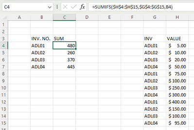
@RohanAbaHK May be you want SUMIFS(). Try-
=SUMIFS($H$4:$H$15,$G$4:$G$15,B4)In case to refer sheet2 use-
=SUMIFS(Sheet2!$H$4:$H$15,Sheet2!$G$4:$G$15,B4)
- Mark as New
- Bookmark
- Subscribe
- Mute
- Subscribe to RSS Feed
- Permalink
- Report Inappropriate Content
Sep 16 2022 01:22 AM
- Mark as New
- Bookmark
- Subscribe
- Mute
- Subscribe to RSS Feed
- Permalink
- Report Inappropriate Content
- Mark as New
- Bookmark
- Subscribe
- Mute
- Subscribe to RSS Feed
- Permalink
- Report Inappropriate Content
Sep 16 2022 01:47 AM
=SUMPRODUCT(($A$4:$A$13=A17)*$B$4:$B$13)Alternatives could be SUMPRODUCT, Power Query and a Pivot Table.

