- Home
- Microsoft 365
- Excel
- Re: VLOOKUP or MATCH - Need Unique Returns on Multiple Finds
VLOOKUP or MATCH - Need Unique Returns on Multiple Finds
- Subscribe to RSS Feed
- Mark Discussion as New
- Mark Discussion as Read
- Pin this Discussion for Current User
- Bookmark
- Subscribe
- Printer Friendly Page
- Mark as New
- Bookmark
- Subscribe
- Mute
- Subscribe to RSS Feed
- Permalink
- Report Inappropriate Content
Feb 01 2023 05:59 AM
Hello All,
Need help on this one. Having issues. I'm trying to summarize a huge list of data. In this huge list of data I need to extract (summarize) extra ingredients used by work order number into one row for that particular workorder. The work orders are itemized by labor hours so they appear in column A multiple times. Some workorders have no extra ingredients.
Here is the data I have:
Column A Column B
Workorder# Extra Ingredients
123 Seeds
456
789 Apple
963
852 Orange
741 Orange
741 Orange
963
123 Seeds
123 Sugar
852
456 Sugar
456
456 Sugar
789
741 Apple
741 Orange
741 CSyrup
741 Apple
What I'm looking for is a formula that puts these values (in another tab) like this:
Column A Column B
Workorder Extra(s)
123 Seeds, Sugar
789 Apple
852 Orange
741 Orange, Apple, CSyrup
456 Sugar
Work orders without any extra ingredients need not be shown in this list. The list is substantial, where maybe there are 100 unique work orders, you'll find those work order number upward in the thousands.
Any help would be greatly appreciated.
- Mark as New
- Bookmark
- Subscribe
- Mute
- Subscribe to RSS Feed
- Permalink
- Report Inappropriate Content
Feb 01 2023 07:00 AM
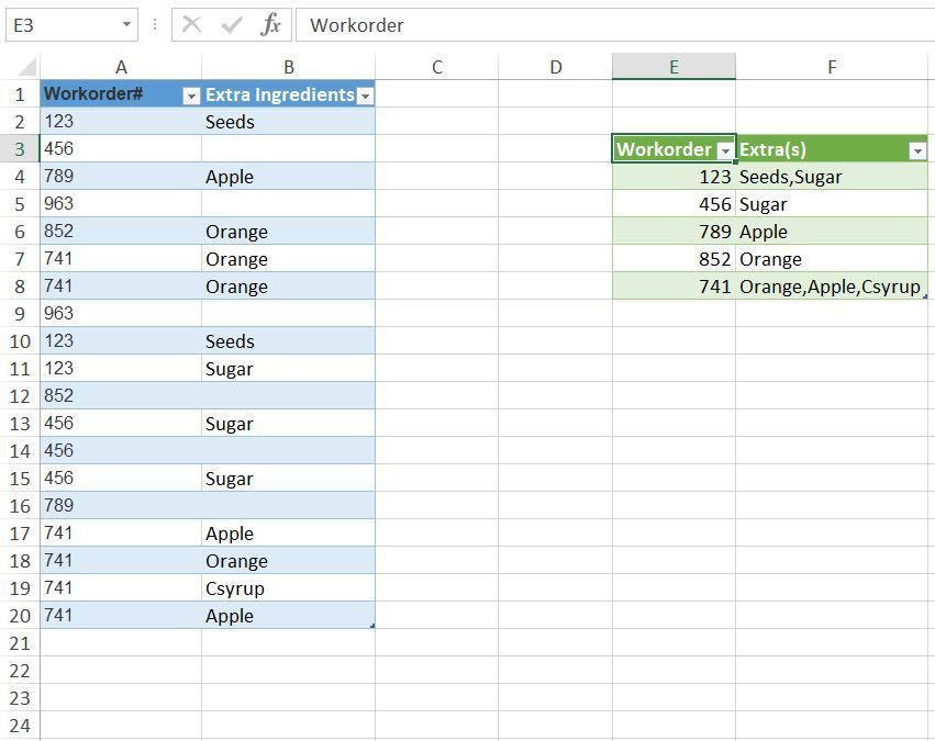
An alternative could be Power Query. In the attached file you can add data into the blue dynamic table and then click in any cell of the green table and right-click with the mouse and select refresh in order to update the green result table.
- Mark as New
- Bookmark
- Subscribe
- Mute
- Subscribe to RSS Feed
- Permalink
- Report Inappropriate Content
Feb 01 2023 07:30 AM
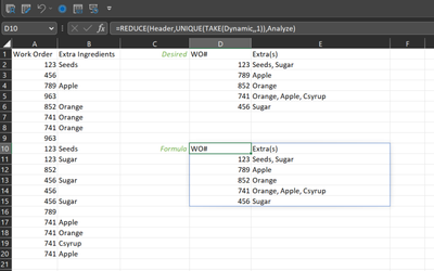
SolutionIf you have access to REDUCE, this may work for you:
'Dynamic' a dynamic range for your data in columns A and B
=LET(arr, Sheet1!$A$2:$B$10000, FILTER(arr, (TAKE(arr, , 1) <> "") * (TAKE(arr, , -1) <> "")))

'Header' - an array constant
={"WO#", "Extra(s)"}

'Analyze' Lambda - to be called within REDUCE. Filters each unique Work Order, obtains the unique ingredients, strings them together, and stacks.
=LAMBDA(a,v,LET(
    WO, TAKE(Dynamic, , 1),
    ingredients, TAKE(Dynamic, , -1),
    filtered, TEXTJOIN(", ", 1, UNIQUE(FILTER(ingredients, WO = v))),
    VSTACK(a, HSTACK(v, filtered))
))

Sheet level formula:
=REDUCE(Header,UNIQUE(TAKE(Dynamic,,1)),Analyze)
- Mark as New
- Bookmark
- Subscribe
- Mute
- Subscribe to RSS Feed
- Permalink
- Report Inappropriate Content
Feb 01 2023 10:50 AM
=REDUCE(Header,UNIQUE(Take(Dynamic,,1)),Analyze(
Analyze is asking for input a,v example: Analyze(a,v). I cannot replicated the below (which you have):
=REDUCE(Header,UNIQUE(TAKE(Dynamic,,1)),Analyze)
- Mark as New
- Bookmark
- Subscribe
- Mute
- Subscribe to RSS Feed
- Permalink
- Report Inappropriate Content
Feb 01 2023 11:02 AM
- Mark as New
- Bookmark
- Subscribe
- Mute
- Subscribe to RSS Feed
- Permalink
- Report Inappropriate Content
Feb 01 2023 12:27 PM
Accepted Solutions
- Mark as New
- Bookmark
- Subscribe
- Mute
- Subscribe to RSS Feed
- Permalink
- Report Inappropriate Content
Feb 01 2023 07:30 AM
SolutionIf you have access to REDUCE, this may work for you:
'Dynamic' a dynamic range for your data in columns A and B
=LET(arr, Sheet1!$A$2:$B$10000, FILTER(arr, (TAKE(arr, , 1) <> "") * (TAKE(arr, , -1) <> "")))

'Header' - an array constant
={"WO#", "Extra(s)"}

'Analyze' Lambda - to be called within REDUCE. Filters each unique Work Order, obtains the unique ingredients, strings them together, and stacks.
=LAMBDA(a,v,LET(
    WO, TAKE(Dynamic, , 1),
    ingredients, TAKE(Dynamic, , -1),
    filtered, TEXTJOIN(", ", 1, UNIQUE(FILTER(ingredients, WO = v))),
    VSTACK(a, HSTACK(v, filtered))
))

Sheet level formula:
=REDUCE(Header,UNIQUE(TAKE(Dynamic,,1)),Analyze)

