Vlookup, or alternative

[cleach86]

Hi, 

I am looking to create a lookup function for a large datasheet probably 120k rows and 10 columns (roughly).

I am looking to lookup using an order number or a drawing number. Sometimes we use the drawing number to find the order number and vice versa. 

The order number consists of 6-10 consecutive digits without spaces. (so this is not a problem)

Drawing numbers consist of 8 digits, a space and a hyphen and number.

examples:

12345678 (this is how we would type the value in)

1234 5678

1234 5678-0

1234 5678-1

1234 5678-2... etc

We usually write the drawing numbers like the first example in the list, but it could be registered in any way I've shown above and the last digit behind the hyphen is not always known.

How should I tackle this issue? Is it possible to do with vlookup, or is it a lot more complex than what this function can do?

Any suggestions are much appreciated!

Thanks

[#2 · Accepted solution]

@cleach86 Perhaps like in the attached file. The formula used is:

=XLOOKUP(D2,VALUE(LEFT(SUBSTITUTE(DrawingNrs," ",""),8)),OrderNrs,"Not found")

where DrawingNrs and OrderNrs are named ranges.

Cannot predict, though, how this will perform on 120K rows,

[#3]

Hi Riny,

Thank you very much for your suggestion!

I will give this a go and let you know how I get on :)

Appreciate your input!

[#4]

Hi,

This seems to be worked just fine! (the sheet actually contains 140k rows) Thank you very much for your help!

I made a small modification to the formula so that I reference to a column on another tab, rather than the name of a column.

Another quick question that you might be able to answer.

What will happen in case of duplicates with this formula?

I am a little unsure if there are any, but just incase there are...

Thanks

[#5]

@cleach86 XLOOKUP, similar to VLOOKUP returns only the first match it finds. 

Since you are using Office 365 you can use FILTER to return all matches to one or multiple criteria. Not sure though how exactly that could be implemented with your specific data.

[#6]

@Riny_van_Eekelen 

Thank you very much for your input, it is appreciated. 

I have got the filter function to work using the serial number and it is returning the values that I want it to show. However, this was the easy part though... 

Is it possible to use the filter function using "jokers", so let's say that "*" is the joker. 

Can I then use the filter function using 1234*5678* to return all the values containing these 8 digits in this order, eventhough they might contain a space or a hyphenation. 

I hope you know what I mean.

[#7]

@cleach86 

I believe you meant "wildcard" when you said "joker" (do you speak Portuguese?). ;)

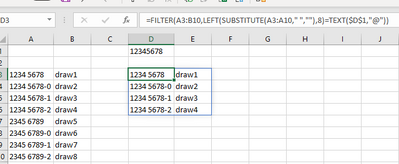
Unfortunately, FILTER does not accept wildcards. You'll have to incorporate LEFT and SUBSTITUTE like in Riny_van_Eekelen first response. This will look something like this:

[#8]

@cleach86 Unlike XLOOKUP, I don't think you can use of wildcards inside the FILTER function. But I may be mistaken. 

However, you could filter for each of the two segments with ISNUMBER and FIND. Such a formula would then look something like this (in the file I attached you earlier).

=FILTER(B4:B8,ISNUMBER(FIND("1234",A4:A8)+FIND("5678",A4:A8,5)))

[#9]

@cleach86 

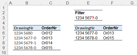
You could exploit the wildcard capability of either COUNTIFS or SEARCH to identify the records to retain.  SEARCH (or FIND) is more straightforward.

= FILTER(Table, ISNUMBER(SEARCH(findText,DrawingNrs)))

[#10]

This is the more complicated approach that uses COUNTIFS to return 1 or 0 for each DrawingNr.  I have used Currying to pass the 'text to find' and the 'text to be searched' separately.

Worsheet Formula
= FILTER(Table, 
      MAP(DrawingNrs, SearchForλ(findText))
  )

SearchForλ 
= LAMBDA(find,
    LAMBDA(searchText, 
        COUNTIFS(searchText, find)
    )
);

Perhaps "less straightforward" understates the challenge?

[#11]

Thank you all for your input!
I got it to work with the wildcards using Peter's method.

This is going to be a great tool that i can start testing now. I don't think that there will be other nasty surprises to take into account.

Thanks again all of you, I hope that you have a nice day!