vlookup multiple values in one cell separated by comma

[Pooyanekooei]

Hello 

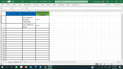
I have a cell that contains multiple data separated by a comma in sheet one (Picture 1)

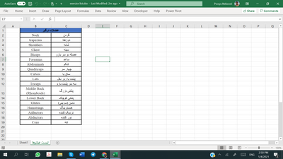
Then I have a table that has data for each of that data in sheet 2 

I want to search the cell C2 that has multiple data in it through the table in sheet 2 and then write them the cell D2 separated by comma again.

[#2 · Accepted solution]

One way I believe you can do that, assuming you have the textjoin function (Ctrl+Shift+Enter after keying into the formula bar):
=TEXTJOIN(", ",TRUE,IF(ISNUMBER(SEARCH('لیست فیلترها'!$B$2:$B$19,C2)),'لیست فیلترها'!$C$2:$C$19,""))

But, I would think the new filter function would also work, if you have it. I personally don't, so this is not tested, but I would try:
=TEXTJOIN(", ",TRUE,FILTER('لیست فیلترها'!$C$2:$C$19,ISNUMBER(SEARCH('لیست فیلترها'!$B$2:$B$19,C2))))

There would be an issue in that you wouldn't get an error if there was an item in C2 that did not appear on the translation table (it would just get left out). So, you might consider adding a check column to confirm the number of items in the original and translated list are the same:

=LEN(C2)-LEN(SUBSTITUTE(C2,",",""))=LEN(D2)-LEN(SUBSTITUTE(D2,",",""))

[#3]

@JMB17  Thank you so much it helps a lot

The only problem is that I want to make the range from 2 to 50 to have a space for future data adding. 

In this case, it showed 0 for empty cells. can we do anything for this one as well?

I mean that in the formula I put the range from B2:B50, but actually I have data until B19 and the rest are empty for now. (In the future I will more data) so the formula showed 0 in the translate cell for each empty cell that is in the main cell. 

I used 

=TEXTJOIN(", ",TRUE,IF(ISNUMBER(SEARCH('لیست فیلترها'!$B$2:$B$50,C2)),'لیست فیلترها'!$C$2:$C$50,""))

actualy I have data until B19. 

[#4]

Try:
=TEXTJOIN(", ",TRUE,('لیست فیلترها'!$B$2:$B$50<>"")*IF(ISNUMBER(SEARCH('لیست فیلترها'!$B$2:$B$50,C2)),'لیست فیلترها'!$C$2:$C$50,""))

[#5]

Thank you so much but this formula is not working at all

[#6]

My apologies. I think I put the additional test for blank in the wrong place in the formula.

=TEXTJOIN(", ",TRUE,IF(('لیست فیلترها'!$B$2:$B$50<>"")*ISNUMBER(SEARCH('لیست فیلترها'!$B$2:$B$50,C2)),'لیست فیلترها'!$C$2:$C$50,""))