VLOOKUP, INDEX and MATCH - can't get them to work

[RobMac14]

Hi,

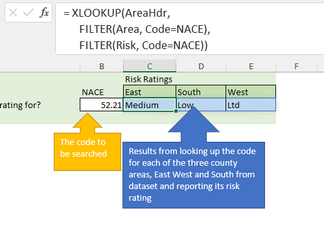
I'm trying to set up an automatic query that when a code is entered a data dump of information is searched to find the risk ratings for that code in 3 different counties.  The data dump will be refreshed regularly so I don't want to spend a lot of time sorting the data dump out before I can run the query to look up the risk ratings.

The code is a four digit code in the format XX.XX ranging from 1.00 to 99.99.  The data dump contains a large amount of information, but all I need to pull out is the risk rating for each of the counties.

I've set up an example of this in the attached spreadsheet, which I hope will illustrate the issue. I can get  VLOOKUP, INDEX and MATCH formulae to return a risk rating for a code but can't seem to figure out how to introduce the county name into them as a third variable to get the three, sometimes different, results.

The code is a four digit code in the format XX.XX ranging from 1.00 to 99.99

I've spent a few hours trying to figure this out.  If anyone can help me or point me in the direct of another function in Excel that will do this for me I'd be very grateful.

Thanks in advance, Rob

[#2 · Accepted solution]

@RobMac14 

You could try this, if you don't have office 365, then you'll need to hit Ctrl+Shift+Enter after keying into the formula bar:

=INDEX('County Data Dump'!$H$2:$H$1846, MATCH(1, ('County Data Dump'!$D$2:$D$1849=$B3)*('County Data Dump'!$B$2:$B$1849=C$2), 0))

[#3]

@RobMac14 

Using 365, you could have

[#4]

hi JMB,
i like the solution, as i am new to this thing. i will be appreciate if you clear my doubt, what this (*) asterisk meant in match function arguments. does it means as AND operator?

[#5]

@harshulz 

Yes, it works as an AND operator.

('County Data Dump'!$D$2:$D$1849=$B3) returns an array of TRUE/FALSE values.
('County Data Dump'!$B$2:$B$1849=C$2) also returns an array of TRUE/FALSE values.
Then, these arrays are multiplied together to get an array of 1's and 0's (TRUE=1 and FALSE=0, so you get a 1 where the elements of both arrays were TRUE).

A simple example, if I were trying to return the value from column C where column A="c" and column B="i"

[#6]

@RobMac14 

=VLOOKUP($B3&C$2,CHOOSE({1,2},'County Data Dump'!$D2:$D1849&'County Data Dump'!$B2:$B1849,'County Data Dump'!$H2:$H1849),2,0)

This formula with VLOOKUP could be an alternative. Enter formula with ctrl+shift+enter if you don't work with Office365 or 2021. 

[#7]

JMB17 - thank you ever so much for replying. Your suggestion worked perfectly and I now have a working spreadsheet to pull out the data I need.

[#8]

Thanks for your reply Peter. I've not used the FILTER function before I will explore it further. Thanks for taking the time to reply.

[#9]

Thanks Quadruple_Pawn for your suggestion. CHOOSE is new to me so another new function to explore. Many thanks.