vlookup for a vertical MAX returning name

[MacTeo84]

hi, 

CUSTOMER CODE	SALES	SALES ADVISOR
123456	3400000	CARLOTTA
123456	300000	MERCO
123456	60000	CATERINA
123456	60000	CATERINA
123456	23500	MATTEO
123456	23500	MATTEO
987654	3436	CATERINA
987654	223344	MERCO
987654	4567	CARLOTTA
987654	3456	MATTEO

hi everyone, 

Given the 'CUSTOMER CODE' with multiple 'SALES' I would like to return the 'SALES ADVISOR' with the best/max 'SALES' value.

i.e. given '987654' -----> 'MERCO'

I tried different vlookup with no success.

Thanks in advance

Matteo

[#2 · Accepted solution]

@MacTeo84 

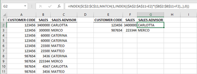
With the customer code in E2, the maximum sales amount in F1 is given by

=MAXIFS($B$2:$B$11,$A$2:$A$11,E2)

and the corresponding sales advisor in G1 is given by

=INDEX($C$2:$C$11,MATCH(1,INDEX(($A$2:$A$11=E2)*($B$2:$B$11=F2),,),0))

These formulas can be filled down, if required.

 

[#3]

@Hans Vogelaar 

Thank you very much!!!!

[#4]

@MacTeo84 

@Hans Vogelaar 's solution is probably simpler!

[#5]

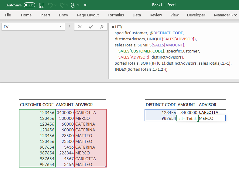
@MacTeo84 And one more. This time with Power Query, as long as you are not on a Mac.

Add sales data to the blue table and refresh the green one to update the summary.

File attached.

[#6]

Irony, of course I'm on Mac... :), but I'll try to apply it on the PC I have at work!!!
Thank you very much!!!!

[#7]

@MacTeo84 Actually, you can add data to the blue table and refresh the green one in this file on a Mac, but you can't edit the queries. You can't even look at them, which makes it quite useless.

[#8]

@Riny_van_Eekelen 

As variant

let
    Source = Excel.CurrentWorkbook(){[Name="Table1"]}[Content],
    #"Grouped Rows" = Table.Group(
        Source, {"CUSTOMER CODE"},
        {{"Count", each  Table.Sort(_,{{"SALES", Order.Descending}}){0} }}
    ),
    #"Expanded Count" = Table.ExpandRecordColumn(
        #"Grouped Rows",
        "Count",
        {"SALES", "SALES ADVISOR"}, {"SALES", "SALES ADVISOR"}
    )
in
    #"Expanded Count"

[#9]

@MacTeo84