Vlookup errors with parenthetic numbers

[Mr_McSquirrelly]

I am trying to make Vlookup find values from a table when values are listed by different names. When I download data from web, my lookup value comes into spreadsheet as (14) Miami (FL), or (10) Texas A&M Aggies. However those same teams are listed in my table as Miami Florida Hurricanes and Texas AM Aggies. VLookup will perform the search and find correct values if I remove the numbers in parentheses, but it causes an error if parenthetic numbers remain in cell. So I need Vlookup to lookup the value (14) Miami (FL) in a table where that value is listed as Miami Florida Hurricanes. The number in parentheses is causing a VLookup N/A# error. Thanks for help in advance.

[#2]

@Riny_van_Eekelen, I tried that, but the problem is the number in parentheses, such as (14) Miami (FL). It's a dynamic data range, so currently the team is listed as Miami (FL) because their rank has changed.

[#3]

@Mr_McSquirrelly But that shouldn't be too difficult to handle. But perhaps I underestimate the problem.

[#4]

@Riny_van_Eekelen @Mr_McSquirrelly 

I tried pq against the list in:

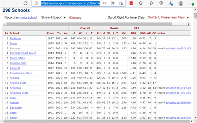
School Index | College Football at Sports-Reference.com

it does not include the actual team name, where referred name in one column and actual team name in another column

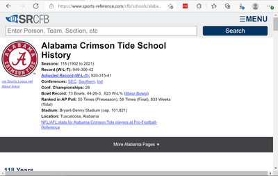
Have to manually click on Alabama for example to get 

so it cannot be down using power query, I tried unless @Mr_McSquirrelly  has a direct link to a table I described above.

cheers

[#5]

@Yea_So 

Thank, Yea So. I've got another problem. Do you think you can solve it?

[#6]

@Mr_McSquirrelly 

lets try and solve it together

[#7]

@Yea_So 

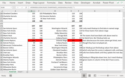
Thank you for your help. Attached spreadsheet. I just need Vlookup to find data for teams with scores in columns B and C in top range and ignore teams with no scores in column B and C. Thanks in advance.

[#8]

@Mr_McSquirrelly 

is my lookup range, A2:F83? or ?? you forgot to mention the lookup range

is my lookup range in the formula correct or not?

[#9]

@Yea_So 

   The range is a named range Teampower_AVGSEASON which has all the season averages of every team. That's why Vlookup is looking up all those numbers in bottom range. It's just the way the data comes from the web. It lists all the teams for the entire season instead of teams that have completed games. I need Vlookup to differentiate between the team with scores in upper range and just look up those teams in named range Teampower_AVGSEASON

[#10]

@Mr_McSquirrelly 

I need to see the layout of Teampower_AVGSEASON

make sure I see the ABCD columns and 1235 rows

Meaning:

so i can see the target ranges

[#11]

@Yea_So 

Here is the entire Spreadsheet. Problem exists in POINTDIF tab

[#12]

@Yea_So 

Maybe I can change the Query for the teams to only bring team names with scores only?

[#13]

@Mr_McSquirrelly 

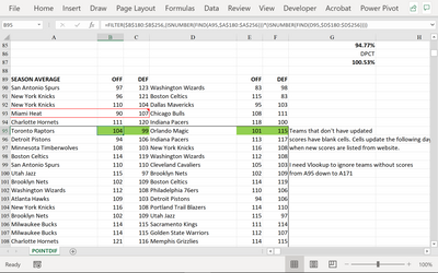
I'm still trying to understand what it is that you are doing in the worksheets, maybe you can help enlighten me with for example:

Toronto raptors formula in this image:

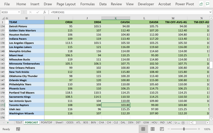
you're looking at column 4 which is:

FORECAST!$H$126:$R$155

which is OAV04 <=== what does OAV04 mean? why is the formula looking for the value in column 4 I need to understand that

[#14]

@Mr_McSquirrelly 

Don't change anything yet!

Maybe I'll need to explain to you excel and formulas.

think of a sheet as a continent

Poindif is a continent and you are in it

Forecast is another continent that is your target you're pointing your missiles at a particular target in Forecast continent so you'll need a map of Forecast continent.

excel is a triangulation equation tool

when you do a look up whether it is VLOOKUP or INDEX+MATCH or some other lookup function, you'll need the exact location of the value "the target"

so you'll triangulate, think of the columns and rows as longitude and latitude.

or you can narrow the triangulation by FILTERING the filter function.

for example:

=FILTER($B$180:$B$256,(ISNUMBER(FIND(A95,$A$180:$A$256)))*(ISNUMBER(FIND(D95,$D$180:$D$256))))

this FILTER function will filter the value range under 2 conditions

condition number 1 it will find the value Toronto raptors in range A180 to A256

condition number 2 it will find the value Orlando Magic in D189 to D256

where it intersects is where the value is "the crosshairs"

do you follow?

so you have 3 elements 1 the range 2 the location of the 2 opposing teams 

because there are 3 Toronto raptors instances in column B and likely 3 instances of Orlando magic as well in column D so in column B has to be true as well as column D so to get the target latitude (horizontal) alignment is between B and D whereas the range is the longitude (vertical alignment) so there's the 1 range, 2 the 1st latitude alignment column B Toronto raptors, 3 the 2nd latitude alignment column D Orlando Magic a triangle.

So the question is what is our Target. I'll need the range column and row and expected value returned so we can decide which function to use whether it be a VLOOKUP, an INDEX+MATCH, or a FIND+FILTER function

[#15]

@Yea_So 

  OAV4 is the Counta Average for the last four scores in a dynamic range. All the team tabs pull data from a website which updates the scores every day after the games are played. OAV4 is the AVERAGE of the last 4 games. It seems complicated. I was just hoping Vlookup could somehow differentiate from the team with scores and the teams with blank scores because I need the average of just the first five teams, and not the average scores of every team in the bottom range.

[#16]

@Mr_McSquirrelly 

that adds a complexity of the formula because:

You know which column the target value is located

because you need 5 values then the FIND+FILTER function is a candidate

because you need the top 5, you're looking at RANK.EQ() or COUNTIFS() or  MAX/MIN or MAXIFS and MINIFS functions as candidates to your solution

so show me the lookup range and explain why this column will be chosen now and if a different column is chosen later on as the game progresses and because why what is the element that changes why it will change later on for example:

with INDEX function we can define multiple ranges to index, and based on the circumstances of whether we're looking for OAV04 or DAV04 etc we can employ a MATCH function to choose which range (area) we will be looking at example:

INDEX([RANGE1],[RANGE2],[RANGE3],,,IF(date()=[some date] is true, then MATCH(OAV04 or DAV04, [ROW RANGE] (will tell match which column/range to look at,[exact match])

something like that. or we can use an INDEX+MATCH+FIND+FILTER kind of solution

where INDEX will tell FIND+FILTER which area to FIND + FILTER then MAXIFS or MINIFS the resulting FILTERED range to find the target.

but if you need all 5 we can employ a table which will list the top 5 and do a VLOOKUP on each. Very complex indeed which will probably involve using power query.

VLOOKUP is only useful in simple one array range, + one latitude parameter if the lookup value is in the middle of the table either employ a VLOOKUP look to the left or INDEX+MATCH because VLOOKUP without the nested IF({1,0} ... can only return values up to the right and the lookup value must be on the left most latitude wise.

[#17]

@Yea_So 

Thank you. I will explore these solutions. 

[#18]

@Mr_McSquirrelly 

I would recommend looking for a solution which would rank and isolate the top 5 dataset:

Ranking Method Choices in Power Query - The Excelguru BlogThe Excelguru Blog

on here, you're project is very challenging i would recommend @Riny_van_Eekelen @Hans Vogelaar @Sergei Baklan @OliverScheurich @L z. they would love to help you with your puzzle especially because you are not stingy sharing your data set.

[#19]

@Yea_So I will contact them. Is it possible to hide the team name in column A when the the score cells in column b and c are blank?

[#20]

@Mr_McSquirrelly 

Worry about that when your project is complete as it may create an unintentional dead end to the complete solution where you will find difficult to find the source of the unintentional bug to your project.

[#21]

@Mr_McSquirrelly DOne! VLOOKUP(MID(A18,6,5),LEFT(Table1,5),2,0)