Vlookup and Sum Help

[RHughes11569]

Can someone help me out with a forumla?

I'm trying to enter an item # on the Lookup sheet of the attached sample and have the YTD Forecast cell in B2 return the sum of the YTD Totals from the Planning Sheet for the matching item # and the forecast rows.

For example, item # 1234 shows up in 3 locations and I need to sum the forecast numbers for those locations.  The total returned should be 2694.  The YTD column for the forecast row is conditional formatted to green if that helps.

[#2 · Accepted solution]

@RHughes11569 Try this in B2 on "Lookup"

=SUMIFS(Planning!D2:D46,Planning!A2:A46,A2,Planning!C2:C46,"Forecast")

[#3]

@RHughes11569 

=SUMIFS(Planning!$D$2:$D$46,Planning!$A$2:$A$46,A2,Planning!$C$2:$C$46,"Forecast")

[#4]

@RHughes11569 

Perhaps PivotTable could be considered as an option

[#5]

@Riny_van_Eekelen That works for me!  I was able to copy your formula into my sheet and then massage it a little to get it to work for my specific worksheet.  Thanks!

[#6]

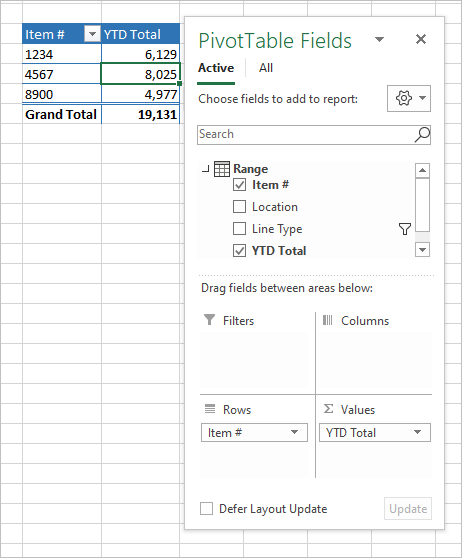
@Sergei Baklan Not that I know a ton about Pivot Tables yet either, but I'm trying to make this as plug & play as possible because some of the people that will be using it know very little about Excel.  I appreciate you helping out though.  I'm definitely learning as I go, so pivot tables are on my list.

[#7]

@RHughes11569 

The minus of PivotTable is that user shall to refresh it after updating the data, formulas do recalculation automatically. At the same time that's quite powerful tool and this option better to keep in mind. Everything depends on concrete situation.