Very odd VLOOKUP problem

[Boblebad]

Hello

I have a very odd problem with the VLOOKUP.

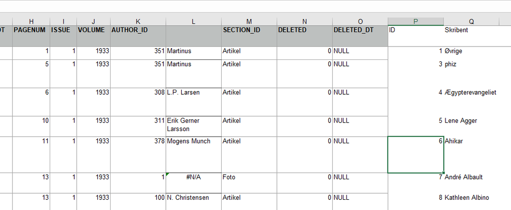
I have a workbook where i have some data for importing to my Wordpress website. I needed to add a column for taxonomy, so i added author name taxonomy and id in columns after the columns with my data for import.

This is my VLOOKUP, which works almost fine: =VLOOKUP(K2;P2:Q712;2;FALSE)

For some wierd reason, the first 5 cells it won't match, but the rest is not a problem. I have checked everything. It's general formatting, have tryed changing it to numbers, nothing changed. Looked for odd extra spaces, none. And when i change the number to get from cell number 6 (which is 7, there's no ID:2) it works just fine. SO it's only the numbers/ID's from the first 5 cells which has the problem. Entering any of them returns "Value not available".

EDIT: And no, it's not the danish characters, there's other authors on the list which works just fine.

What can be the problem ?

All the best

Carsten

[#2]

@Boblebad 

Change the formula in L2 to

=VLOOKUP(K2;$P$2:$Q$712;2;FALSE)

Then fill down.

[#3]

Thank you Hans. it worked :)

Can you tell me why ?

I really don't understand it, because i got it from a guide on how to do it. I have seen others where they use $ in front of all columns and cell-number. And why did it give me such a wierd error ?

I tried moving the numbers around and found out that if i deleted the first 1-entry and moved that maybe ten places down the list, then it work, but only for two row, and then the error again for the rest. I then loaded another file with more rows to test it on a completely new set of data; Same result. - But, number 46 fell of the wagon too this time :o

[#4 · Accepted solution]

@Boblebad 

In your original formula in L2 =VLOOKUP(K2;P2:Q712;2;FALSE), the references to K2 and to P2:Q712 are relative. this means that Excel will adjust them automatically when you fill or copy L2 to other cells.

In L3 it becomes =VLOOKUP(K3;P3:Q713;2;FALSE), in L4 it will be =VLOOKUP(K4;P4:Q714;2;FALSE) etc.

The change from K2 to K3, K4, ... is exactly what you want, but the change from P2:Q712 to P3:Q713 etc. is not. It causes the first IDs to drop out of the range.

To prevent this, we add $ signs. They make the reference absolute. Excel will not change an absolute reference when you fill or copy the cell with the formula to other cells.

So the formula in L2 =VLOOKUP(K2;$P$2:$Q$712;2;FALSE) will become =VLOOKUP(K3;$P$2:$Q$712;2;FALSE) in L3, and =VLOOKUP(K4;$P$2:$Q$712;2;FALSE) in L4, etc.

The reference to K2 changes, as desired, but the reference to $P$2:$Q$712 does not change.

The easiest way to change P2:Q712 to $P$2:$Q$712 is to select it in the formula and to press F4.

For more info, see Switch between relative, absolute, and mixed references 

[#5]

@Hans Vogelaar Thank you for the explanation :)

I saw that the Q-number added up, and thought that it might be a problem in some way, but couldn't see anything happen to that column. So therefor i didn't suspect it to be that which caused the problems in the L-column.