VBA Code to Automatically Copy and Paste a Range of Data if the Criteria is Met

[ABro_1111]

Hi,

I am looking for some help with a copy and paste code. 

I want excel to determine if the values in one column is less than the values in another and if so, copy/paste those rows of data into another sheet. Since more information would be added to the original data set, I also want excel to copy/paste the new data into the next available row on the other sheet. 

The codes I wrote to check if the values in one column < the values in another column weren’t running so I decided to create a helper column that runs the formula and returns True/False. So my current VBA code is written to see if “True” is in that range and to copy those rows of data and paste them where I want after resizing it to omit that helper column. 

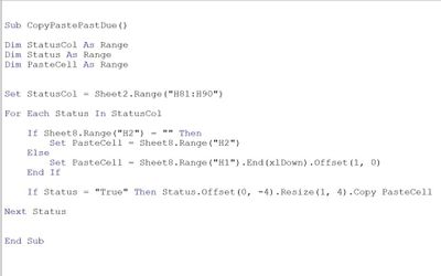
Unfortunately, when I run the code it is only pasting the last row that tests true (but in that PasteCell I can see it run through all the rows that are True and it completes the paste only of the last row that is True.) 

I’ve added an image of the code for reference. 

Could someone please help me spot why it’s not pasting the desired range or help me rewrite another code that will? 

Thanks!!

 

 

[#2]

@ABro_1111 

You don't need a macro to accomplish this, not if you have a current version of Excel (>=2021) or a subscription to Microsoft 365.

This formula, using the FILTER function, does the task. See the attached spreadsheet for the working example. And you can add rows of data.

=FILTER(Table1,Table1[Actual]<Table1[Expected],"none")

Here's a link that explains the FILTER function.

[#3]

Hi @mathetes ,

Unfortunately, I have an older version of excel and plan on sending the file to someone who has an older version as well. I tried a good old INDEX/MATCH/ROWS function to accommodate for not having the FILTER function and it didn’t work either it came up saying “#REF!” or “NA” or “VALUE” or only pastes a value from one cell. 

[#4 · Accepted solution]

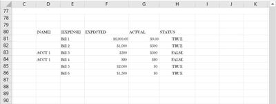
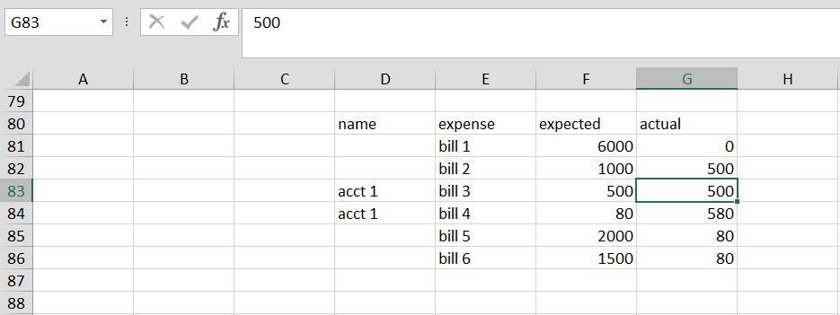
@ABro_1111 

=IFERROR(INDEX(Sheet2!D$81:D$86,SMALL(IF(Sheet2!$F$81:$F$86>Sheet2!$G$81:$G$86,ROW(Sheet2!$A$81:$A$86)-80),ROW($A1))),"")

Without VBA you can try this formula. The formula has to be entered as an arrayformula with ctrl+shift+enter if one doesn't work with Office 365 or Excel 2021. In the example the formula is in cell H2 of sheet8 and filled across range H2:K8.

Sheet2:

Sheet8:

 

[#5]

@OliverScheurich

Thank you!

It works perfect. If I have any follow questions, I’ll be back!

[#6]

I am trying to modify the function to apply it to something else. In this case, I am trying to copy and paste the range of cells were the value is greater than “>0”. Unfortunately, in each modification of the function, it isn’t working like the recommendation.

One column contains a list and in another column is a SUMIF function that corresponds to the list column. I’m trying to use the function to only copy the values in that range where the SUMIF column has values “>0” and paste them on another sheet.

I’ve tried looking to see if other people have posted a similar question and gotten an answer but haven’t found anything replicable.

Again, I am open to a code that could automatically run as new data is added.

[#7]

@ABro_1111 

Could you attach a screenshot of your data (without sensitive information) and of the expected result?

[#8]

@OliverScheurich 

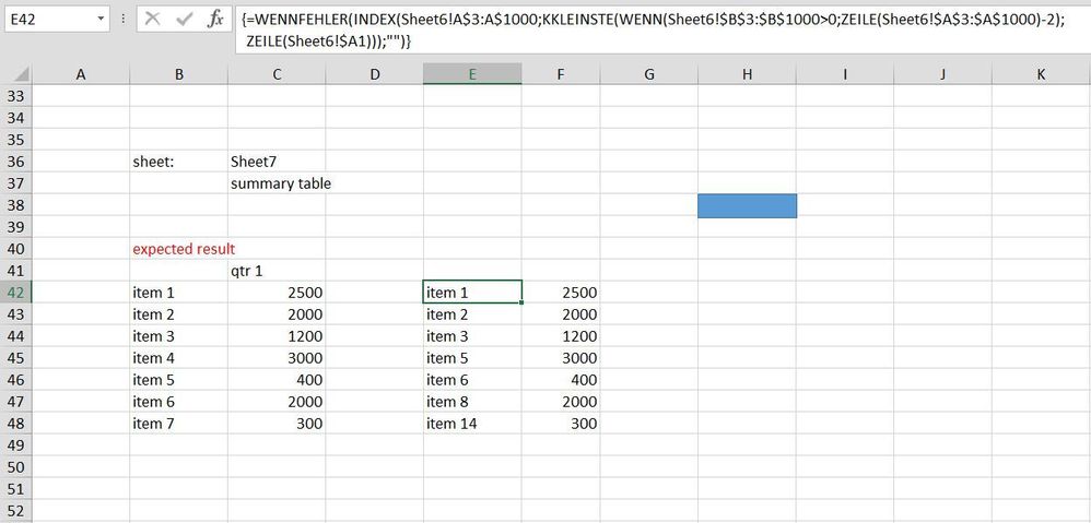
Sure! So I've designed a simplified mockup and attached it for you. Hope it makes sense. But I'll explain it a bit more below.

On one sheet (named"Sidework") I have tons of data which is where my drop-down lists are derived from.

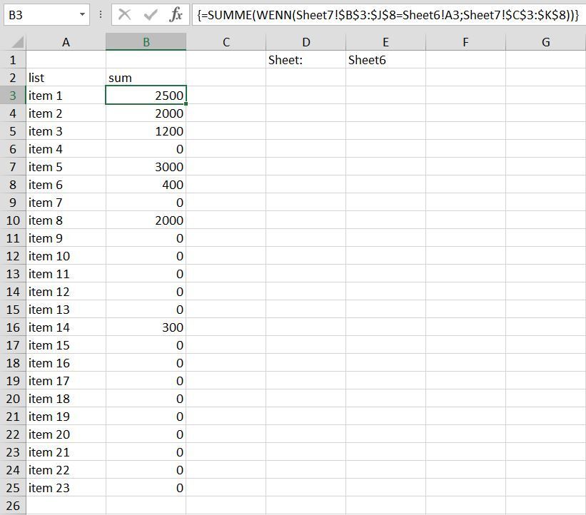
I then used another sheet named "Sheet6" to house data. The first column is a direct reference to the list from the "Sidework" sheet so that they are updated simultaneously. The second column contains the SUMIF formula

My summary sheet, "Sheet7" is where the values and data are updated. So for each person, I can select the item from the drop-drown list created, and insert how much they've earned from it. (This is what my SUMIF function is referencing.)

This is where I need help:
At another location on the same sheet, I want to display the data in another way. Showing the total earned per item rather than per person. But, I want excel to filter the data from Sheet6 and just copy and paste the range of data (just values and format) where the values in column B are greater than 0.

So I tried to modify the function you gave me, by applying it to the data on Sheet6. But, I haven't had success (I think it's because the entire data set is technically a function.) Similar to the first example, my data is dynamic, so I need something that works with changing data.

*Note: I'm open to all suggestions as well. Thank you

[#9]

@ABro_1111 

Thank you for the detailed explanation. You can try this formula which must be entered as an arrayformula with ctrl+shift+enter if one doesn't work with Office 365 or Excel 2021.

=IFERROR(INDEX(Sheet6!A$3:A$1000,SMALL(IF(Sheet6!$B$3:$B$1000>0,ROW(Sheet6!$A$3:$A$1000)-2),ROW(Sheet6!$A1))),"")

The formula is in cell E42 of Sheet7 and filled across range E42:F51. The formula can be filled down and the ranges in the formula can be adapted from e.g. Sheet6!A$3:A$1000 to Sheet6!A$3:A$20000.

An alternative could be these lines of code. In the attached file you can click the button in cell H38 of Sheet7 to run the macro.

Sub summary()

Dim i, j, k As Integer

Sheets("Sheet7").Range("H42:I1048576").Clear
j = Sheets("Sheet6").Range("A" & Rows.Count).End(xlUp).Row
k = 42
For i = 3 To j
If Sheets("Sheet6").Cells(i, 2).Value > 0 Then
Sheets("Sheet7").Cells(k, 8).Value = Sheets("Sheet6").Cells(i, 1).Value
Sheets("Sheet7").Cells(k, 9).Value = Sheets("Sheet6").Cells(i, 2).Value
k = k + 1
Else
End If

Next i

End Sub

In cell B3 of Sheet6 i've entered a shorter formula which must be entered as an arrayformula with ctrl+shift+enter if one doesn't work with Office 365 or Excel 2021. The ranges of the formula can be adapted as required.

=SUM(IF(Sheet7!$B$3:$J$8=Sheet6!A3,Sheet7!$C$3:$K$8))

[#10]

@OliverScheurich 

Once again, thank you!