Use Formula for Cell Reference - Example: Sliding Window Average

[Stomachbuzz]

Is it possible to use a formula in a cell reference?

For example, 'sum of the last 12 cells'. So the cell address might be =SUM($C$(ROW(THIS.CELL)-12):C19)

I know this gets into relative cells, but this is a larger exercise to calculate a sliding window average. The issue is the starting conditions.

Let's say I want to calculate average income over the last 12 months.

How can I make it 'auto-generate friendly' when there are less than 12 months? I.E for the first 11 months.

In a table, the first cell would be: =SUM($C$2:C2)/1 (because there's only 1 month so far)

Second cell would be... =SUM($C$2:C3)/2 (because 2 months)

...

11th would be =SUM($C$2:C12)/11

Later cells would then all be uniform with denominator of 12.

=SUM($C10:C21)/12

In short, I want the starting cell reference to be '12 cells up' unless that would be outside of the table, with the ending cell being the current cell. Then the denominator would be the similar scheme.

So far I've gotten, for rows, =MIN(ROW(A21)-1,12) which effectively takes the 'low-select' of the row value.
If greater than 12, denominator = 12, else denominator = row-1

[#2]

@Stomachbuzz 

If you have 365, presuming the data is in column A. You could use:

=LET(rng,A1:A100,blanks,COUNTBLANK(rng),dynamic,DROP(rng,-blanks),Last_12,TAKE(dynamic,-12),AVERAGE(Last_12))

If there's not 12 numbers to average yet, TAKE will grab what's there and it will be averaged.

[#3]

@Stomachbuzz 

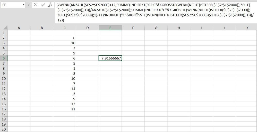
=IF(COUNT($C$2:$C$2000)<12,SUM(INDIRECT("C2:C"&LARGE(IF(NOT(ISBLANK($C$2:$C$2000)),ROW($C$2:$C$2000)),1)))/COUNT($C$2:$C$2000),SUM(INDIRECT("C"&LARGE(IF(NOT(ISBLANK($C$2:$C$2000)),ROW($C$2:$C$2000)),1)-11):INDIRECT("C"&LARGE(IF(NOT(ISBLANK($C$2:$C$2000)),ROW($C$2:$C$2000)),1)))/12)

This formula returns the expected result in my sheet. Enter the formula with ctrl+shift+enter if you don't work with Office365 or 2021.

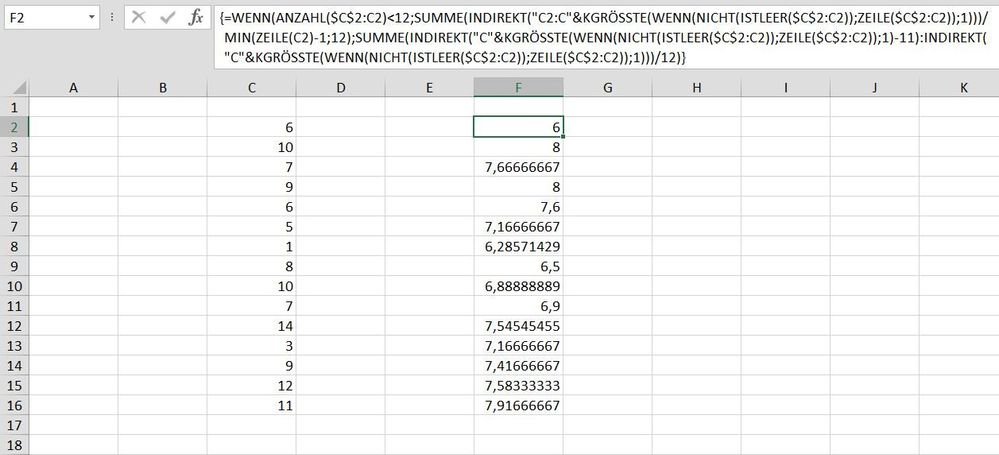
=IF(COUNT($C$2:C2)<12,SUM(INDIRECT("C2:C"&LARGE(IF(NOT(ISBLANK($C$2:C2)),ROW($C$2:C2)),1)))/MIN(ROW(C2)-1,12),SUM(INDIRECT("C"&LARGE(IF(NOT(ISBLANK($C$2:C2)),ROW($C$2:C2)),1)-11):INDIRECT("C"&LARGE(IF(NOT(ISBLANK($C$2:C2)),ROW($C$2:C2)),1)))/12)

This formula returns the results if you want to copy the formula down from row 2. Enter the formula with ctrl+shift+enter if you don't work with Office365 or 2021.

[#4]

Thank you for these replies! It is appreciated