Unexpected Pivot Table Header Changes by itself

[GordH42]

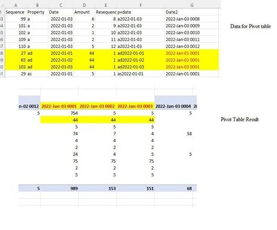
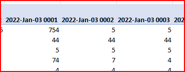
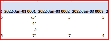
Hi,  I have created a pivot data but the header column data seems to have changed when compared to the actual raw data. Below is a picture of the raw data where the Property is the row, Date2 is the columns and Amount is the data value. With reference to the highlighted rows, the Date2 is showing Jan-01, Jan-02 and Jan03. You would expect to see this in the Pivot table. However, in the following pic of the pivot tabe (see highlighted column headings) all the dates appears to be Jan-03? You can see the corresponding data of 44 appear there but some how the data for the headings changed?  Any help please.

 

[#2]

@GordH42 

Just refreshed and it works. Did you change PivotTable manually?

By the way, on each Excel version/platform you are?

[#3]

I figure it out or at least partially. When I highlighted the FULL columns (not just the raw data area but all the blank rows) for the pivot area, it comes up with this error. When I highlighted only the data area for the pivot table, it is ok. It's reproducible.

Table Range: $A:$G gives this odd error.
Table Range: $A$1:$G$115 gives the right answer.

Thank you all and especially Detlef for all the help. Sorry for the newbie error.




https://www.dropbox.com/scl/fi/9caowtiad1lw1pskeqtng/Weird-pivot-table-result-3.xlsx?dl=0&rlkey=wjdn...

[#4]

To answer your question. No did not change the data manually. If you look at my latest version uploaded in dropbox, the headings are now correct but also the data in now in a different spot. I would have had to change both the headings and the data manual to get to this weird result. And no point in that. But have to ask.

[#5]

@GordH42 

I can't reproduce

Open the file

after refresh

[#6]

@Sergei Baklan   Hi.  I have uploaded a video buried in a powerpoint showing the two highlighting options and the differeing results. One where I highlight the entire columns and secondly, where I only highlight the data area. Plus I have added the excel file with these results in dropbox links below.

https://www.dropbox.com/scl/fi/s8vm9fddjvnrohibnmsf5/Reproducible-Pivot-differences.pptx?dl=0&rlkey=...

https://www.dropbox.com/scl/fi/xon12pt3u01fxglj0qi34/Weird-pivot-table-result-5.xlsx?dl=0&rlkey=dhvj...

[#7]

@GordH42 

I see, thank you. Now I can reproduce. So, the problem if only you select entire columns. Don't know what is exact reason, something is wrong in calculation chain. Workarounds could be

1) Refresh PivotTable after creating, with data change and on file opening.

2) Creating PivotTable add data to data model

3) In source data change Resequence formula on

=COUNTIFS($B$2:$B2, B2, $C$2:$C2, C2 )

4) Or change that formula on

=IF(B2&C2<>B1&C1,1,1+E1)

5) Convert source data to structured table and build PivotTable on it

With any of above it (or combination of them) works, at least in my case.

[#8]

Thanks for the options. I have not tried your suggestions. I think I will just stick with making sure that only the data area is highlighted for the pivot table and no thighlight the columns.

Thanks to all.