Turn off condition formatting of a cell based on different cell

[GeneP]

Good Morning, I have a formula running in cell K11 based on other cells (J11 and current date)  that provides a number, then conditional formatting to highlight the cell based on the value. 

Next I wish to use information from a 3rd cell (M11) to turn off the formula and formatting in K11, Once anything is present it M11, K11 goes blank with no highlight. 

Likely this is a new formatting rule --> Use a formula to determine which cells to format, that's as for as I get. Can anyone help with this?  Thanks....

[#2]

@GeneP 

You may check if it is something in M11 or not by checking length of the value of this cell.

To return empty string to K11 you shall update your current formula for K11 with above condition.

Not to highlight K11 in such case you may add another conditional formatting rule on first position which check M11 length and apply Fill No color format K11.

[#3]

@Sergei Baklan  Ok 

1--take my formula that I am generating the value for K11 (=Days(J11, J3(the cell containing the current date))---then add to this formula to have it also check M11 so that it checks for anything there. if anything then the formula yields no valve and therefore no formatting kicks in. If any thing is there in M11 then go ahead and do the calculation and my formatting happens?? Can you provide any sample language? I don't know how to right it. Thanks....

[#4]

@GeneP 

Perhaps we may generate concrete formula if you provide small sample file.

[#5]

@Sergei Baklan So from the attached file you can see I am tracking the progress for receiving a submittal. I have a date that I need to receive the document. I am comparing today's date to the need by date, and displaying the number of days remaining. I am them color coding the cell as the days grow shorter. Once I log a date into M11 announcing it has been received I need the tracking occurring in K11 to stop. That cell needs to display no number and return to white background. 

So is that maybe having the formula in K11 first check for a value in M11 first, if valve-->stop, if no value proceed to run=DAYS(J11-J3). Conditional formatting I could do from there, no valve no formatting, whatever number --> formatting.

Thanks....

[#6 · Accepted solution]

@GeneP 

I updating the formulas a bit starting from row 12 and till end of the range.

In I12

=IF($G12="","",$G12-($H12+$I12)*7)

it shows empty cells in column J if no req date (col G)

In K12

=IF(OR($M12<>"",$G12=""),"",J12-TODAY())

It returns empty cell if no req date (column G) or order is closed (date in column M)

Conditional formatting:

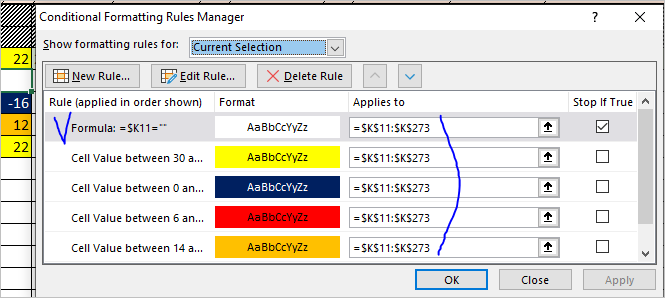
All rules are expanded on entire range (not to generate bunch of new rules applying cell by cell with Format Painter) and one more rule on the top with "no color" if the cell is blank

Please check in attached file.

[#7]

@Sergei Baklan  Thanks much for this. I am studying the formula trying to see what you have done. It is doing what I wanted, trying to learn something new.  Again Thank you.....

[#8]

@GeneP , you are welcome. Please ask if something is unclear.